Time Series Forecasting Foundations: The Moving Average Process and MA(q) Model
The Moving Average Model is a regression technique used to model time series data by incorporating a linear combination of past values, similar to the Autoregressive process. However, unlike the Autoregressive process that models based on lagged values, the MA model utilizes previous errors to model the data.
When a moving average process underlies time series data, we can model the data as a linear combination of the average/mean of the time series, the current error, and past errors. Mathematically, we can represent this process as:
$$ y_t = \mu + \epsilon_t + \theta_1 \epsilon_{t-1} + ... + \theta_q \epsilon_{t-q} $$
where:
$\mu$: is the average of the series
$\theta:$ is the error term
Dataset Visualization and Assessment
The dataset used in this note contains the prices of a publicly traded stock at the daily level. The code below reads and visualizes the data to assess trends and understand the nature of the dataset.
import numpy as np
import pandas as pd
import matplotlib.pyplot as plt


%matplotlib inline
%config InlineBackend.figure_format = 'retina'
data = pd.read_csv('data/stock_data.csv')
data.head()| data | price | |
|---|---|---|
| 0 | 2021-04-03 | 59.44 |
| 1 | 2021-04-04 | 61.67 |
| 2 | 2021-04-05 | 63.03 |
| 3 | 2021-04-06 | 63.99 |
| 4 | 2021-04-03 | 64.09 |
plt.figure(figsize=(10, 4))
plt.plot(data.date, data.price, linewidth=1, marker='o', markersize=2)
plt.title('Daily Closing Price')
plt.xlabel('date')
plt.ylabel('price in USD $')
plt.show()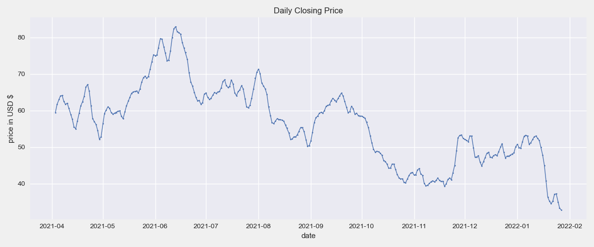
Stationarity and Differencing
Like the AR(p) model, the MA(q) model assumes stationarity of the time series. Judging visually, the nature of the time series suggests that is not stationary. However, we must test it to determine stationarity.
from statsmodels.tsa.stattools import adfuller

statistic, p_value = adfuller(data.price)[:2]

if p_value < .05:
    print(f'p_value: {p_value} Time Series is Stationary')
else:
print(f'p_value: {p_value} Time Series is not Stationary')p_value: 0.6251206124726647 Time Series is not Stationary
As expected from the time series view, the data is not stationary. At this point, differencing is a good transformation to apply and test for stationarity.
data['diff'] = data.price.diff()

statistic, p_value = adfuller(data['diff'].dropna())[:2]

if p_value < .05:
    print(f'p_value: {p_value} \nTime Series is Stationary')
else:
print(f'p_value: {p_value} \nTime Series is not Stationary')p_value: 2.2582368454232396e-12 Time Series is Stationary
Visualizing Original Data and Differenced Data
fig = plt.figure(figsize=(10, 6))

fig.add_subplot(211)
plt.plot(data.date, data.price, linewidth=1, marker='o', markersize=2)
plt.title('Daily Closing Price')
plt.xlabel('date')
plt.ylabel('price in USD $')


fig.add_subplot(212)
plt.plot(data.date, data['diff'] )
plt.title('Differences Series at Lag = 1')
plt.xlabel('date')
plt.ylabel('differenced price lag=1')

plt.tight_layout()
plt.show()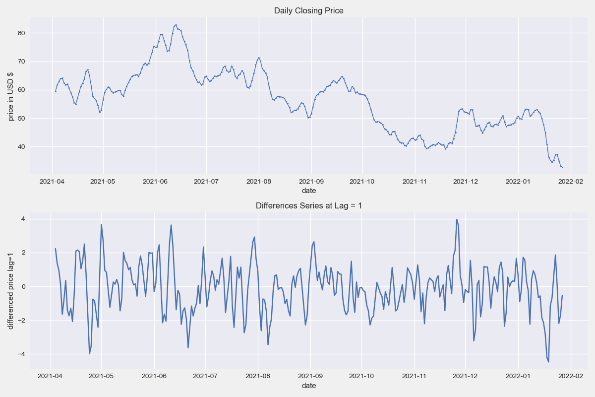
Autocorrelation Plots
A helpful determinant of significant lags for the MA(q) model is the autocorrelation plot. With a moving average process, we expect the significant autocorrelation lags to drop more abruptly after some lag q.
from statsmodels.graphics.tsaplots import plot_acf

plt.rc("figure", figsize=(9,4))
plot_acf( data['diff'].dropna(), lags=20, auto_ylims=True)
plt.show()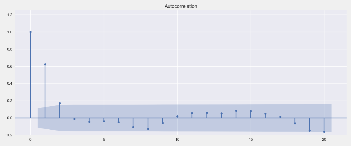
In this case, we notice that the autocorrelation drops after lag 2. This means that we can use a moving average with $q=2$. Note that this is not a strict requirement and depends on the significance threshold set.
Fitting MA(q) Model
For training the MA(q) model, I will implement two different routines. Both approaches will use SARIMAX() with the same order but will differ slightly in implementation:
- 1. The first approach will fit the model against all the data and run predictions. The data is therefore a full train set.
- 2. The second approach will fit iteratively, predicting one point at a time and using every past event
The implementation of both these two approaches is available below:
from statsmodels.tsa.statespace.sarimax import SARIMAX

# differenced series
diff_series = data[['date', 'diff']].dropna()
diff_series.set_index('date', inplace=True)

# MA ORDER
order = (0, 0, 3)
1. Using full dataset as training set
# Training on full data
ts_model = SARIMAX( diff_series, order=order, freq='d')
results = ts_model.fit(disp=False)
predictions = results.get_prediction().predicted_mean[:]
2. Using an iterative train set and predicting one outcome at a time
# train and test sets
data_size = len(diff_series)
train_size = int(.75 * data_size)
test_size = data_size - train_size


iterative_predictions = []

### Iterative Training
for i in range(train_size, data_size+1):

    #  MODEL FITTING
    iterative_model = SARIMAX( diff_series[:i], order=order)
    iterative_model_results = iterative_model.fit(disp=False)

    # PREDICT LAST VALUE AND APPEND TO PREDICTIONS
    iterative_predictions.extend( iterative_model_results.get_prediction(0, i+1).predicted_mean.iloc[-1:])
Fit Model Results
diff_series['one_pass_fit'] = predictions
diff_series['iterative_fit'] = diff_series.iloc[:train_size, 0].tolist() + iterative_predictions[:-1]
diff_series.head()| diff | one_pass_fit | iterative_fit | |
|---|---|---|---|
| date | |||
| 2021-04-04 | 2.23 | 0.000000 | 2.23 |
| 2021-04-05 | 1.36 | 1.403364 | 1.36 |
| 2021-04-06 | 0.96 | 0.368542 | 0.96 |
| 2021-04-07 | 0.10 | 0.565433 | 0.10 |
| 2021-04-08 | -1.65 | -0.242266 | -1.65 |
plt.figure(figsize=(9,4))
plt.plot(diff_series.index, diff_series['diff'], label='differenced_series')
plt.plot(diff_series.index, diff_series.one_pass_fit, label='training_fit')
plt.plot(diff_series.index[train_size:], diff_series.iloc[train_size:, 2], label='iterative_fit')
plt.title('Differenced Series MA(2): Actual vs. Predicted')
plt.legend()
plt.show()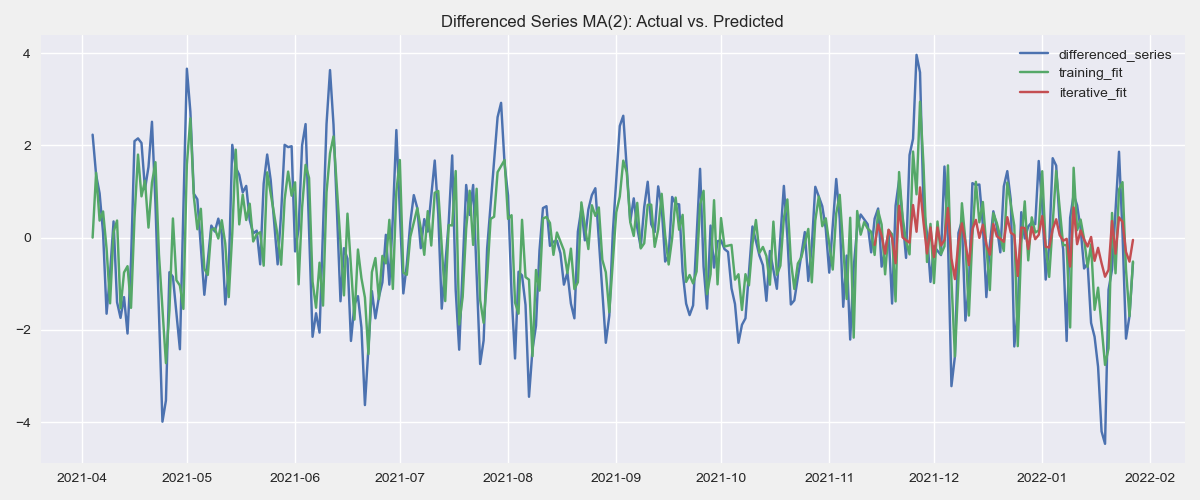
Converting Differenced Values to Actuals
The forecast is on differenced values of the original price and needs to be converted into its original form to be of any good use. The code below implements the conversion which is simply a cumulative sum.
full_data = pd.merge( left=data, right=diff_series, on='date', how='outer')
full_data.head()| data | diff | one_pass_fit | iterative_fit | |||
|---|---|---|---|---|---|---|
| 0 | 2021-04-03 | 59.44 | NaN | NaN | NaN | NaN |
| 1 | 2021-04-04 | 61.67 | 2.23 | 2.23 | 0.000000 | 2.23 |
| 2 | 2021-04-05 | 63.03 | 1.36 | 1.36 | 1.403364 | 1.36 |
| 3 | 2021-04-06 | 63.99 | 0.96 | 0.96 | 0.368542 | 0.96 |
| 4 | 2021-04-07 | 64.09 | 0.10 | 0.10 | 0.565433 | 0.10 |
 # initializing first values of the series
full_data.iloc[0, 4] = full_data.iloc[0, 1]
full_data.iloc[0, 5] = full_data.iloc[0, 1]

# converting to real numbers
full_data['one_pass_predictions'] = full_data['one_pass_fit'].cumsum()
full_data['iterative_predictions'] = full_data['iterative_fit'].cumsum()
Finally, let's visualize the actual price and the predictions
plt.figure(figsize=(9,3))
plt.plot(full_data.index, full_data.price, label='actual_price')
plt.plot(full_data.index, full_data.one_pass_predictions, label='one_pass_prediction')
plt.plot(full_data.index[train_size:], full_data.iterative_predictions[train_size:], label='iterative_prediction')

plt.ylabel('price')
plt.xlabel('date')

plt.title('Actual vs. Predicted Price')
plt.legend()
plt.show()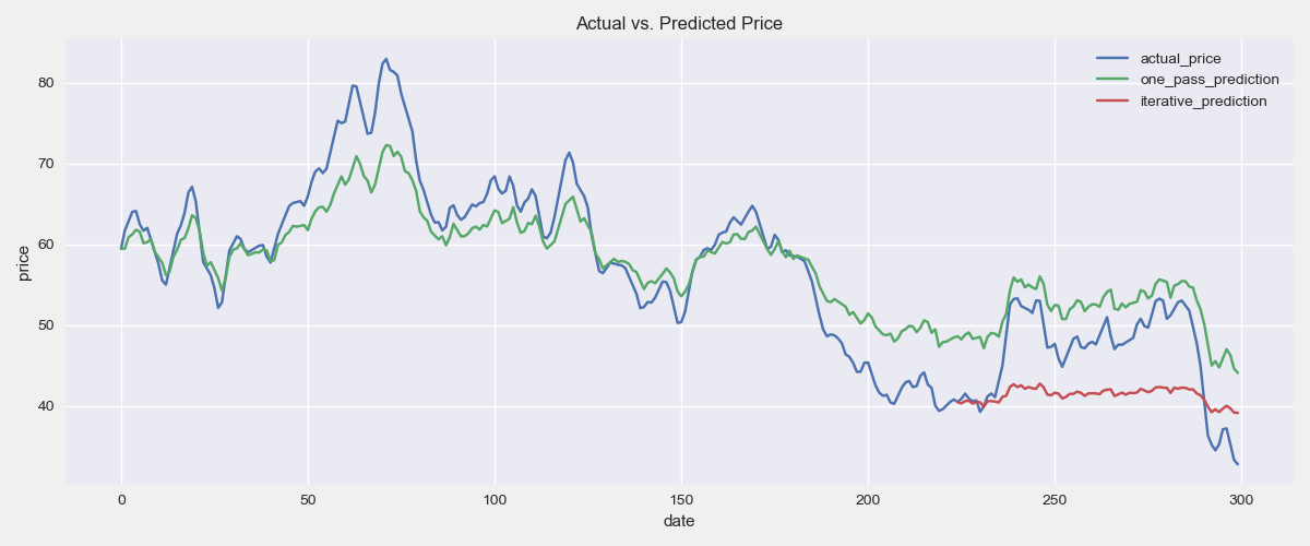
Beyond the MA(q) Model
As the purpose of this note is to introduce the core components of the moving average model as a standalone, I will conclude it here. However, it is important to note that the MA model alone may not fully capture the underlying behavior of the time series. To enhance the model's results and performance, incorporating an AR component is recommended.