Detecting Pneumonia on Chest XRay Images
This note develops an End-2-End pipeline and deep learning model to predict the presence of Pneumonia on chest X-ray images. The dataset is available on Kaggle through this link: Kaggle Labeled Chest X-ray Images
The pipeline will follow the following steps:
- 1. Chest X-Ray Data Exploration and Visualization
- 2. Building Pytorch Dataset, DataLoader, and Transformations
- 3. Building Convolutional Network Architecture
- 4. Model Training and Evaluation Routine
1. Chest X-Ray Data Extraction - File Structure
To begin, download the datasets and save them in the current directory. Within the chest_xray folder, there will be test and train subfolders each containing folders of normal vs pneumonia x-ray images. The folder structure would look like below.
!tree -d
.
└── chest_xray
    ├── test
    │   ├── NORMAL
    │   └── PNEUMONIA
    └── train
        ├── NORMAL
        └── PNEUMONIA

7 directories
Exploring the Chest X-Ray Images
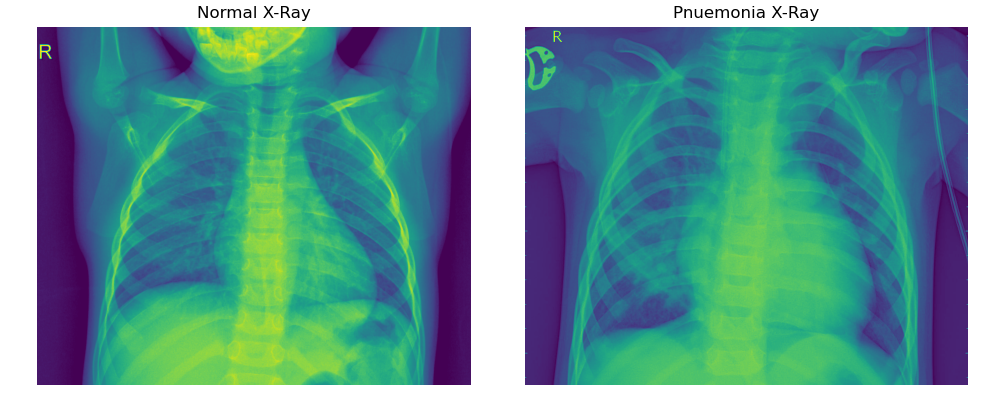
Visualizing the chest X-ray images helps us gain key insights into the datasets and helps us design our transformations. We can get a sense of the image dimensions, channels, composition, and any interesting transformation that may be necessary to develop a complex sample set for modeling. The code below draws a few samples of train and test chest X-ray images for visualization.
import os
import numpy as np
import matplotlib.pyplot as plt
import matplotlib.image as mpimg


%matplotlib inline
%config Inline.Backend.figure_format = 'retina'
train_path = os.path.join('chest_xray', 'train')
test_path = os.path.join('chest_xray', 'test')
train_normal_images = os.listdir( os.path.join(train_path, 'NORMAL'))
train_pneumonia_images = os.listdir( os.path.join(train_path, 'PNEUMONIA'))
# negative and positive samples
samples_n, samples_p = np.random.randint( len(train_normal_images), size=1), np.random.randint(len(train_pneumonia_images), size=1),
samples_n, samples_p(array([244]), array([3106]))
fig = plt.figure( figsize=(10,4))

img = mpimg.imread( os.path.join(train_path, 'NORMAL', train_normal_images[samples_n[0]]) )
fig.add_subplot(121)
plt.imshow(img)
plt.title('Normal X-Ray')
plt.axis('off')


img = mpimg.imread( os.path.join(train_path, 'PNEUMONIA', train_pneumonia_images[samples_n[0]]) )
fig.add_subplot(122)
plt.imshow(img)
plt.title('Pnuemonia X-Ray')
plt.axis('off')


plt.tight_layout()
Chest X-ray Image Transforms and Augmentation
One apparent observation of the chest X-ray images is that each image has varying dimensions. Some X-ray images have more pixels than others. Similarly, in the above images, the X-ray on the left contains more of the patient's facial skeletal component than the one on the right. We can also observe that the hands of the patient on the left are raised while those on the right are lateral. These are only two samples, but we can expect a varying number of differences across the total train and test set
One thing that is common across all images is that the chest remains at the center of the image. This is a useful feature because we could remove any unwanted features (such as the face and hands) by implementing a CenterCrop transformation, which will retain the chest area.
from torchvision import transforms

transform = transforms.Compose([ transforms.Resize(224),
                                 transforms.CenterCrop(224),
                                 transforms.ColorJitter(brightness=0.10,  contrast=0.1, saturation=0.10, hue=0.1),
                                 transforms.RandomHorizontalFlip(),
                                 transforms.RandomRotation(10) ])
To demonstrate the example output, let's run a sample image against the transform:
from PIL import Image

samples_n = np.random.randint( len(train_normal_images), size=1)
sample_img = Image.open( os.path.join(train_path, 'NORMAL', train_normal_images[samples_n[0]]) )
transformed_img = transform(sample_img)
fig = plt.figure( figsize=(10,4) )

fig.add_subplot(121)
plt.imshow(sample_img),
plt.title('Original X-Ray')

fig.add_subplot(122)
plt.imshow(transformed_img)
plt.title('Transformed X-Ray')

plt.tight_layout()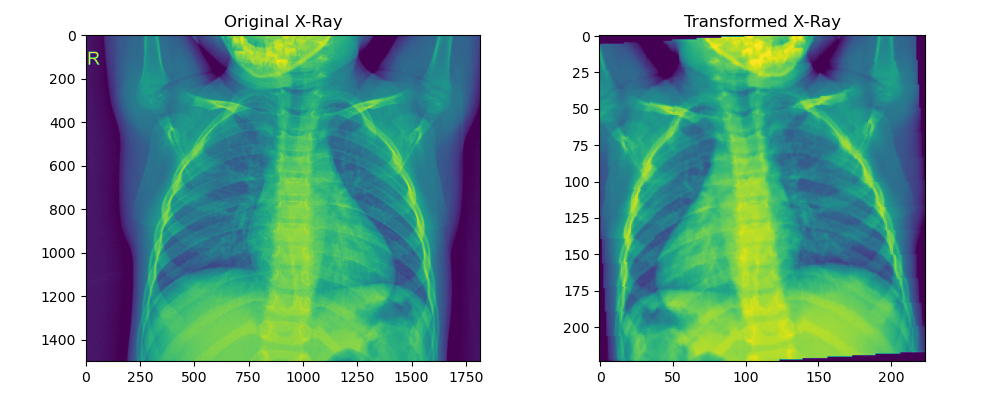
2. Creating a PyTorch Dataset, DataLoader, and Transformations
Before we can define a model, we need to generate a dataset and a dataloader object for the train and test images. To achieve this, we use torchvision.ImageFolder, which expects the folder structure to be set up as we have done for the train and test sets. We will then apply the transformations directly to the dataset, including some light augmentation through random rotation and horizontal flips.
from torchvision import datasets
from torch.utils.data import Dataset, DataLoader

transform = transforms.Compose([ transforms.Resize(224),
                                    transforms.CenterCrop(224),
                                    transforms.ColorJitter(brightness=0.10, contrast=0.1, saturation=0.10, hue=0.1),
                                    transforms.RandomHorizontalFlip(),
                                    transforms.RandomRotation(10),
                                    transforms.ToTensor(),
                                    transforms.Normalize([ 0.485, 0.456, 0.405], [ 0.229, 0.224, 0.225 ]) ])


# Creating  datasets
train_data = datasets.ImageFolder( train_path, transform=transform  )
test_data = datasets.ImageFolder( test_path, transform=transform )

# Creating data loaders for batch training
train_loader = DataLoader( train_data, batch_size=16, shuffle=True )
test_loader = DataLoader( test_data, batch_size=16, shuffle=False)

train_data.classes, train_data.class_to_idx(['NORMAL', 'PNEUMONIA'], {'NORMAL': 0, 'PNEUMONIA': 1})train_data
Dataset ImageFolder
    Number of datapoints: 5232
    Root location: chest_xray/train
    StandardTransform
Transform: Compose(
               Resize(size=224, interpolation=bilinear, max_size=None, antialias=None)
               CenterCrop(size=(224, 224))
               ColorJitter(brightness=[0.9, 1.1], contrast=[0.9, 1.1], saturation=[0.9, 1.1], hue=[-0.1, 0.1])
               RandomHorizontalFlip(p=0.5)
               RandomRotation(degrees=[-10.0, 10.0], interpolation=nearest, expand=False, fill=0)
               ToTensor()
               Normalize(mean=[0.485, 0.456, 0.405], std=[0.229, 0.224, 0.225])
           )
sample_idx = np.random.randint( len(train_data) ,size=1)
plt.imshow(train_data[sample_idx[0]][0].permute(1, 2, 0))
plt.title(f"Sample Tensor Image: # {sample_idx[0]}")
plt.show()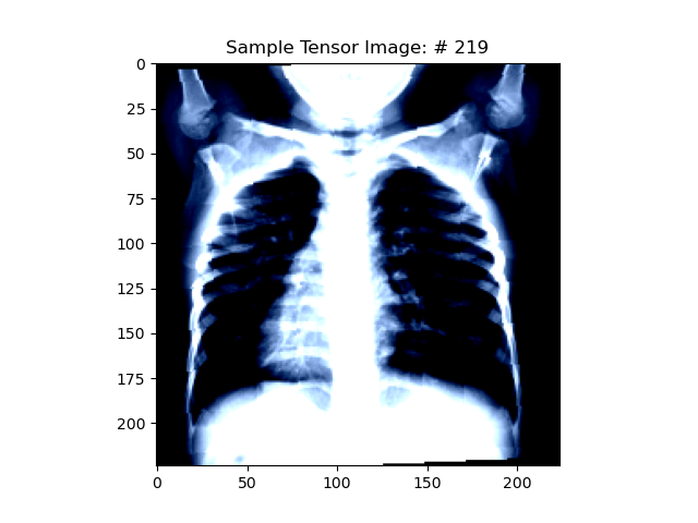
3. Building Convolutional Network Architecture
The model architecture, named PneumoniaNet, consists of a sequence of convolutional layers organized in 11 blocks. Each block applies a convolutional operation with ReLU activation and batch normalization, followed by a max pooling operation. The output of the convolutional layers is then passed through an average pooling layer and a final convolutional layer with kernel size 4. The output is flattened and passed through a logarithmic softmax function to obtain the final classification probabilities.
import torch
import torch.nn as nn
from torchsummary import summary
import torch.nn.functional as F

class PneumoniaNet(nn.Module):

    def __init__(self):
        super(PneumoniaNet, self).__init__()

        # Generating Features
        self.features = nn.Sequential(
            # Block 1
            nn.Conv2d( in_channels=3, out_channels=32, kernel_size=3, stride=1),
            nn.ReLU(inplace=True),
            nn.BatchNorm2d(32),
            nn.MaxPool2d(2, 2),

            # Block 2
            nn.Conv2d( in_channels=32, out_channels=16, kernel_size=3, stride=1),
            nn.ReLU(inplace=True),
            nn.BatchNorm2d(16),
            nn.MaxPool2d(2, 2),

            # Block 3
            nn.Conv2d( in_channels=16, out_channels=10, kernel_size=1, stride=1),
            nn.ReLU(inplace=True),
            nn.BatchNorm2d(10),
            nn.MaxPool2d(2, 2),

            # Block 4
            nn.Conv2d( in_channels=10, out_channels=10, kernel_size=3, stride=1),
            nn.ReLU(inplace=True),
            nn.BatchNorm2d(10),


            # Block 5
            nn.Conv2d( in_channels=10, out_channels=32, kernel_size=1, stride=1),
            nn.ReLU(inplace=True),
            nn.BatchNorm2d(32),

            # Block 6
            nn.Conv2d( in_channels=32, out_channels=10, kernel_size=1, stride=1),
            nn.ReLU(inplace=True),
            nn.BatchNorm2d(10),

            # Block 7
            nn.Conv2d( in_channels=10, out_channels=10, kernel_size=3, stride=1),
            nn.ReLU(inplace=True),
            nn.BatchNorm2d(10),

            # Block 8
            nn.Conv2d( in_channels=10, out_channels=32, kernel_size=1, stride=1),
            nn.ReLU(inplace=True),
            nn.BatchNorm2d(32),

            # Block 9
            nn.Conv2d( in_channels=32, out_channels=10, kernel_size=1, stride=1),
            nn.ReLU(inplace=True),
            nn.BatchNorm2d(10),


            # Block 10
            nn.Conv2d( in_channels=10, out_channels=14, kernel_size=3, stride=1),
            nn.ReLU(inplace=True),
            nn.BatchNorm2d(14),


            # Block 11
            nn.Conv2d( in_channels=14, out_channels=16, kernel_size=3, stride=1),
            nn.ReLU(inplace=True),
            nn.BatchNorm2d(16),
        )

        self.avg_pool = nn.AvgPool2d(kernel_size=4)
        self.output_layer = nn.Sequential(
            nn.Conv2d(in_channels=16, out_channels=2, kernel_size=4)
        )
        # self.classifier = nn.Sequential(
        #      # Hidden Layer
        #      nn.Linear(16 * 4 * 4, 64),
        #      nn.ReLU(inplace=True),
        #      nn.Dropout(.5),

        #      # Output Layer
        #      nn.Linear(64, 1),
        # )


    def forward(self, x):
        x = self.features(x)
        x = self.avg_pool(x)
        x = self.output_layer(x)
        x = x.view(-1, 2)

        return F.log_softmax(x, dim=-1)
use_cuda = torch.cuda.is_available()
device = torch.device("cuda" if use_cuda else "cpu")
model = PneumoniaNet().to(device)

summary(model, input_size=(3, 224, 224))
----------------------------------------------------------------
    Layer (type)               Output Shape         Param #
================================================================
        Conv2d-1         [-1, 32, 222, 222]             896
          ReLU-2         [-1, 32, 222, 222]               0
   BatchNorm2d-3         [-1, 32, 222, 222]              64
     MaxPool2d-4         [-1, 32, 111, 111]               0
        Conv2d-5         [-1, 16, 109, 109]           4,624
          ReLU-6         [-1, 16, 109, 109]               0
   BatchNorm2d-7         [-1, 16, 109, 109]              32
     MaxPool2d-8           [-1, 16, 54, 54]               0
        Conv2d-9           [-1, 10, 54, 54]             170
         ReLU-10           [-1, 10, 54, 54]               0
  BatchNorm2d-11           [-1, 10, 54, 54]              20
    MaxPool2d-12           [-1, 10, 27, 27]               0
       Conv2d-13           [-1, 10, 25, 25]             910
         ReLU-14           [-1, 10, 25, 25]               0
  BatchNorm2d-15           [-1, 10, 25, 25]              20
       Conv2d-16           [-1, 32, 25, 25]             352
         ReLU-17           [-1, 32, 25, 25]               0
  BatchNorm2d-18           [-1, 32, 25, 25]              64
       Conv2d-19           [-1, 10, 25, 25]             330
         ReLU-20           [-1, 10, 25, 25]               0
  BatchNorm2d-21           [-1, 10, 25, 25]              20
       Conv2d-22           [-1, 10, 23, 23]             910
         ReLU-23           [-1, 10, 23, 23]               0
  BatchNorm2d-24           [-1, 10, 23, 23]              20
       Conv2d-25           [-1, 32, 23, 23]             352
         ReLU-26           [-1, 32, 23, 23]               0
  BatchNorm2d-27           [-1, 32, 23, 23]              64
       Conv2d-28           [-1, 10, 23, 23]             330
         ReLU-29           [-1, 10, 23, 23]               0
  BatchNorm2d-30           [-1, 10, 23, 23]              20
       Conv2d-31           [-1, 14, 21, 21]           1,274
         ReLU-32           [-1, 14, 21, 21]               0
  BatchNorm2d-33           [-1, 14, 21, 21]              28
       Conv2d-34           [-1, 16, 19, 19]           2,032
         ReLU-35           [-1, 16, 19, 19]               0
  BatchNorm2d-36           [-1, 16, 19, 19]              32
    AvgPool2d-37             [-1, 16, 4, 4]               0
       Conv2d-38              [-1, 2, 1, 1]             514
================================================================
Total params: 13,078
Trainable params: 13,078
Non-trainable params: 0
----------------------------------------------------------------
Input size (MB): 0.57
Forward/backward pass size (MB): 46.18
Params size (MB): 0.05
Estimated Total Size (MB): 46.81
----------------------------------------------------------------
Model Training and Test Evaluation Routine
The training and evaluation of this model will happen concurrently against each training batch. This way, I will be able to track training and test error rates and accuracy. For the training and parameter estimation, I use a $ \text {learning rate} = .01 $ with the Negative Log Loss function.
train_losses, test_losses = [], []
train_accuracy, test_accuracy = [], []
from tqdm import tqdm
def train(model, device, train_loader, optimizer, epoch):
model.train()
progress_bar = tqdm(train_loader)
correct, processed = 0, 0
for batch_idx, (data, target) in enumerate(progress_bar):
data, target = data.to(device), target.to(device)
optimizer.zero_grad()
y_pred = model(data)
loss = F.nll_loss(y_pred, target)
train_losses.append(loss)
# Back Prop
loss.backward()
optimizer.step()
pred = y_pred.argmax(dim=1, keepdim=True)
correct += pred.eq(target.view_as(pred)).sum().item()
processed += len(data)
progress_bar.set_description( desc=f"Loss = {loss.item()}, Batch_id = {batch_idx}, Accuracy={100*correct/processed:0.2f}" )
train_accuracy.append(100*correct/processed)
def test(model, device, test_loader):
model.eval()
test_loss = 0
correct = 0
with torch.no_grad():
for data, target in test_loader:
data, target = data.to(device), target.to(device)
output = model(data)
test_loss += F.nll_loss(output, target, reduce='sum').item()
pred = output.argmax(dim=1, keepdim=True)
correct += pred.eq(target.view_as(pred)).sum().item()
test_loss /= len(test_loader.dataset)
test_losses.append(test_loss)
print(" \n Test Set: Average Loss: {:.4f}, Accuracy: {}/{}({:.2f}%)\n".format( test_loss, correct, len(test_loader.dataset), 100 * correct/len(test_loader.dataset)))
test_accuracy.append(100 * correct/len(test_loader.dataset))import torch.optim as optim
from torch.optim.lr_scheduler import StepLR
# parameters
learning_rate = .01
optimizer = optim.SGD( model.parameters(), lr=learning_rate, momentum=.9)
scheduler = StepLR(optimizer, step_size=6, gamma=.5) # Implements learning rate decay
epochs = 20

for epoch in range(epochs):
    print(f"Epoch: {epoch}")
    train(model, device, train_loader, optimizer, epoch)
    scheduler.step()
    print("Current Learning Rate: ", optimizer.state_dict()['param_groups'][0]['lr'])
test(model, device, test_loader)Epoch: 0 Loss = 0.18759295344352722, Batch_id = 326, Accuracy=94.90: 100%|██████████| 327/327 [03:34<00:00, 1.52it/s] Current Learning Rate: 0.01 Test Set: Average Loss: 0.0362, Accuracy: 504/624(80.77%) Epoch: 1 Loss = 0.24247106909751892, Batch_id = 326, Accuracy=94.94: 100%|██████████| 327/327 [03:35<00:00, 1.52it/s] Current Learning Rate: 0.01 Test Set: Average Loss: 0.0337, Accuracy: 519/624(83.17% . . . Epoch: 19 Loss = 0.0961175337433815, Batch_id = 326, Accuracy=97.46: 100%|██████████| 327/327 [03:35<00:00, 1.52it/s] Current Learning Rate: 0.00125 Test Set: Average Loss: 0.0280, Accuracy: 540/624(86.54%)
Visualizing Model Performance
The model training is complete. We can now visualize the training and evaluation losses and accuracy.
train_losses_list = [  float(x.cpu().detach().numpy()) for x in train_losses  ]
train_accuracy_list = [ x for x in train_accuracy ]
test_losses_list = [x for x in test_losses]
test_accuracy_list = [x for x in test_accuracy]
fig, ax = plt.subplots(2, 2, figsize=(16,8))
ax[0,0].plot(train_losses_list)
ax[0,0].set_title('Training Loss')
ax[1,0].plot(train_accuracy_list)
ax[1,0].set_title('Train Accuracy')
ax[0,1].plot(range(1,21),test_losses_list)
ax[0,1].set_title('Test Losses')
ax[1,1].plot(range(1,21), test_accuracy_list)
ax[1,1].set_title('Test Accuracy')
plt.show()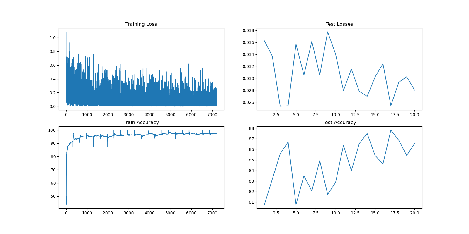
During the 20 epochs and across different batches, the model has shown improvement over time without apparent overfitting on the test set. The accuracy has consistently increased with periods of calibration in different epochs. These improvements may be attributed to the learning rate decay set up in the training routine. Although the current results are satisfactory for the exercise, further experimentation with different layer configurations, data augmentation techniques, and longer training durations may lead to even better results.