Pencil Sketch Image Conversion in Python

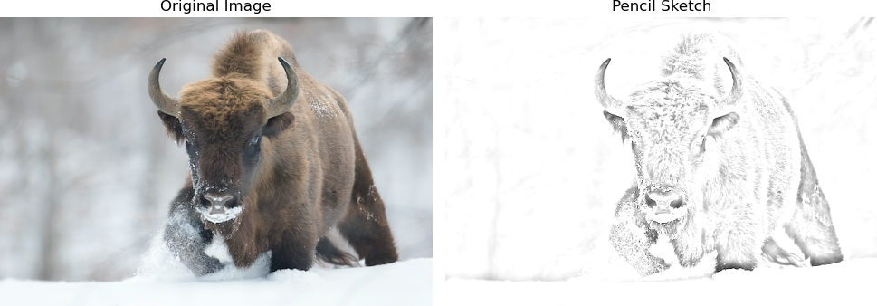
Social Media apps like Instagram and Snapchat offer a number of filters to create realistic effects on video and image content. One such filter is a pencil sketch which turns an original image into a pencil sketch image. This note demonstrates the implementation steps for such conversion using Python and OpenCV libraries.

Pencil Sketch Implementation Steps

There are four basic implementation steps to turn an image into a pencil sketch image.

1. 1. Conversion from Color to Grayscale
2. 2. Inverting an image i.e. swap black and white images for the full image
3. 3. Apply Gaussian Blur on inverted image
4. 4. Divide original_grayscale image to the inverted blur image #3

Below is a step-by-step implementation of the Pencil Sketch with OpenCV

Step 0: Reading and Visualizing the dataset

Before we implement the Pencil Sketch above, let's read and visualize the original image

import cv2
import numpy as np 
import matplotlib.pyplot as plt

%matplotlib inline
%config InlineBackend.figure_format = 'retina'

img = cv2.imread('data/bison.jpg')
img = cv2.cvtColor(img, cv2.COLOR_BGR2RGB)


fig = plt.figure(figsize=(5,5))
plt.imshow(img)
plt.axis('off')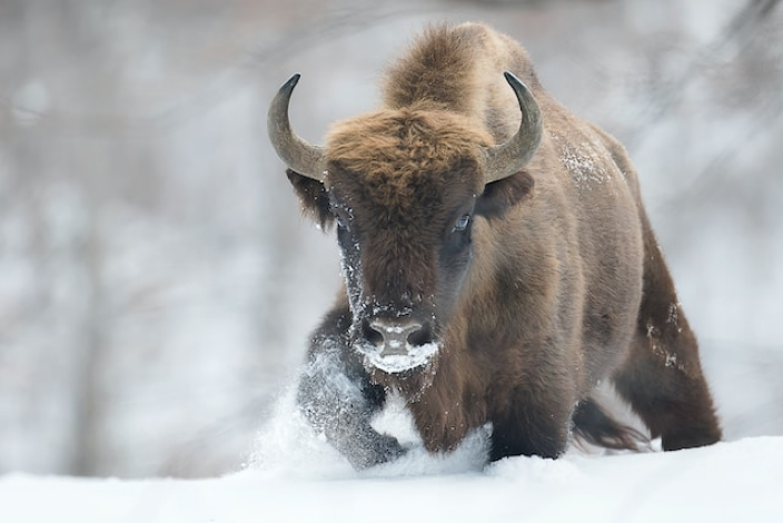

Step 1: Convert Color Image to Gray Scale

Grayscale conversion is a standard practice to allow for more complex operations while limiting impact on original channels. We apply the same conversion here as well.

img_gray = cv2.cvtColor(img, cv2.COLOR_RGB2GRAY)

fig = plt.figure(figsize=(5,5))
plt.imshow(img_gray, cmap="gray")
plt.axis('off')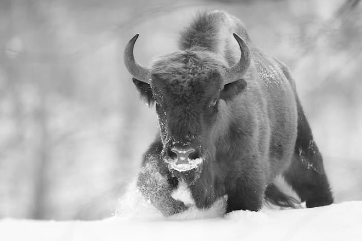

Step 2: Invert the Grayscale Image

The process of inverting the grayscale image pixel values is straightforward. We subtract each pixel value from 255. As a result, white pixels which are of value 255 will turn to zero (therefore becoming black) and vice versa. The result is seen below for our image.

img_inverse_gray = 255 - img_gray

fig = plt.figure(figsize=(5,5))
plt.imshow(img_inverse_gray, cmap="gray")
plt.axis('off')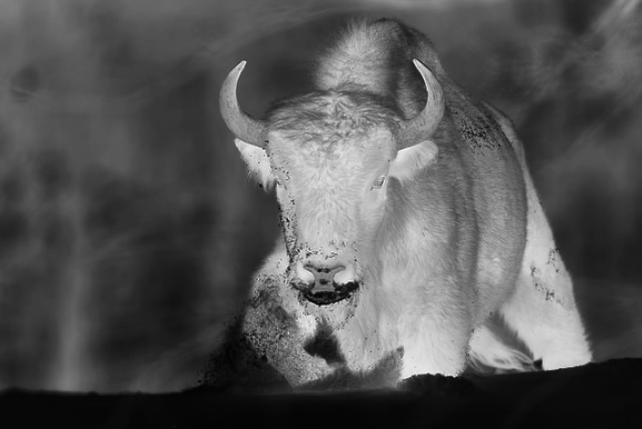

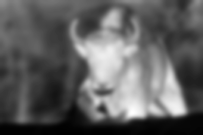
Step 3: Implement Gaussian Blur

The Gaussian Blur has the effect of normalizing the pixels in an image following the distribution. Broadly, it is used to smooth an image by reducing edges that have sharp pixel differentials.

This step has an impact on the final image. It turns out that the bigger the Gaussian blur kernel, the stronger the pencil sketch in the end. For this demonstration, I use a gaussian kernel of 41 by 41 and a standard deviation of 7

gaussian_kernel_dimension = (41, 41)
gaussian_kernel_sd = 7
img_inverse_gray_blur = cv2.GaussianBlur(img_inverse_gray, gaussian_kernel_dimension, gaussian_kernel_sd)
        
fig = plt.figure(figsize=(5,5))
plt.imshow( img_inverse_gray_blur, cmap="gray")
plt.axis('off')
    

Step 4: Divide the Gray Image by the Inverse of Gaussian Blur image

Finally, we take the original image and divide it by the inverse of the blurred image above limiting the pixel values to 255 with the scale argument $(scale=256)$

sketch = cv2.divide(img_gray, 255 - img_inverse_gray_blur, scale = 256)

fig = plt.figure(figsize=(5,5))
plt.imshow( sketch, cmap="gray")
plt.axis('off')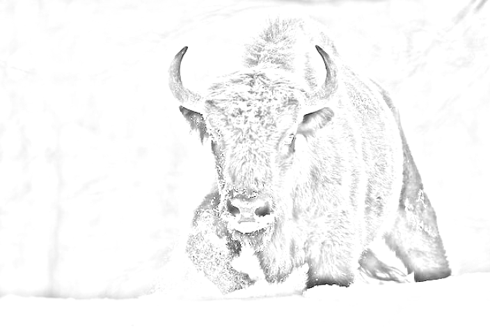

That's it. Give it a try.