Part 2: Building a 68-Facial Keypoint Detection with PyTorch
In Part I,we explored the dataset, created a custom Dataset class, and implemented data augmentation techniques.
In this second part, we will focus on building the Convolutional Neural Network (CNN) architecture, setting up
the training pipeline using PyTorch, and training the model on a Apple Silicon Mac using the
Let begin by importing the necessary libraries.
import os
import torch
import torch.nn as nn
import torch.optim as optim
from torch.utils.data import Dataset, DataLoader
from torchvision import transforms, utils
import pandas as pd
import numpy as np
import matplotlib.pyplot as plt
import cv2

# Check for MPS availability
device = torch.device('mps' if torch.backends.mps.is_available() else 'cpu')
print(f'Using device: {device}')Using device: mps
The Data Pipeline Recap
We re-implement the Dataset and Transform classes from Part 1 to ensure our notebook is fully functional.
class FacialKeypointsDataset(Dataset):
    def __init__(self, root_dir, csv_file, transform=None):
        self.root_dir = root_dir
        self.keypoints_frame = pd.read_csv(csv_file)
        self.transform = transform

    def __len__(self):
        return len(self.keypoints_frame)

    def __getitem__(self, idx):
        img_name = os.path.join(self.root_dir, self.keypoints_frame.iloc[idx, 0])
        image = cv2.imread(img_name)
        image = cv2.cvtColor(image, cv2.COLOR_BGR2RGB)
        if image.shape[2] == 4:
            image = image[:, :, 0:3]

        keypoints = self.keypoints_frame.iloc[idx, 1:].to_numpy().astype('float').reshape(-1, 2)
        sample = {'image': image, 'keypoints': keypoints}
        if self.transform:
            sample = self.transform(sample)
        return sample

class Normalize(object):

    def __call__(self, sample):
        image, keypoints = sample['image'], sample['keypoints']
        image_copy = cv2.cvtColor(image, cv2.COLOR_RGB2GRAY)
        image_copy = image_copy/255.0
        keypoints_copy = (keypoints - 100)/50.0
        return {'image': image_copy, 'keypoints': keypoints_copy}

class Rescale(object):
    def __init__(self, output_size):
        self.output_size = output_size

    def __call__(self, sample):
        image, keypoints = sample['image'], sample['keypoints']
        h, w = image.shape[:2]
        new_h, new_w = (self.output_size, self.output_size)
        img = cv2.resize(image, (new_w, new_h))
        keypoints = keypoints * [new_w / w, new_h / h]

        return {'image': img, 'keypoints': keypoints}

class ToTensor(object):
    def __call__(self, sample):
        image, keypoints = sample['image'], sample['keypoints']
        if len(image.shape) == 2:
            image = image.reshape(image.shape[0], image.shape[1], 1)

        image = image.transpose((2, 0, 1))
        return {'image': torch.from_numpy(image).float(), 'keypoints': torch.from_numpy(keypoints).float()}
Model Architecture
We define a CNN with four convolutional layers followed by three fully connected layers. Dropout is used to prevent overfitting.
class Net(nn.Module):
    def __init__(self):
        super(Net, self).__init__()
        self.conv1 = nn.Conv2d(1, 32, 5)
        self.pool = nn.MaxPool2d(2, 2)
        self.conv2 = nn.Conv2d(32, 64, 3)
        self.conv3 = nn.Conv2d(64, 128, 3)
        self.conv4 = nn.Conv2d(128, 256, 3)
        self.fc1 = nn.Linear(256 * 12 * 12, 1000)
        self.fc2 = nn.Linear(1000, 500)
        self.fc3 = nn.Linear(500, 136)
        self.dropout = nn.Dropout(0.2)

    def forward(self, x):
        x = self.pool(torch.relu(self.conv1(x)))
        x = self.pool(torch.relu(self.conv2(x)))
        x = self.pool(torch.relu(self.conv3(x)))
        x = self.pool(torch.relu(self.conv4(x)))
        x = x.view(x.size(0), -1)
        x = self.dropout(torch.relu(self.fc1(x)))
        x = self.dropout(torch.relu(self.fc2(x)))
        x = self.fc3(x)
        return x

model = Net().to(device)
print(model)Net( (conv1): Conv2d(1, 32, kernel_size=(5, 5), stride=(1, 1)) (pool): MaxPool2d(kernel_size=2, stride=2, padding=0, dilation=1, ceil_mode=False) (conv2): Conv2d(32, 64, kernel_size=(3, 3), stride=(1, 1)) (conv3): Conv2d(64, 128, kernel_size=(3, 3), stride=(1, 1)) (conv4): Conv2d(128, 256, kernel_size=(3, 3), stride=(1, 1)) (fc1): Linear(in_features=36864, out_features=1000, bias=True) (fc2): Linear(in_features=1000, out_features=500, bias=True) (fc3): Linear(in_features=500, out_features=136, bias=True) (dropout): Dropout(p=0.2, inplace=False) )
Dataset Instance
Now, let's generate instances of our dataset and transforms.
data_transform = transforms.Compose([Rescale(224), Normalize(), ToTensor()])
train_dataset = FacialKeypointsDataset(root_dir='data/training/', csv_file='data/training_frames_keypoints.csv', transform=data_transform)
train_loader = DataLoader(train_dataset, batch_size=32, shuffle=True)
Loss and Optimizer
The next step is to pick the Loss function and the optimizer
criterion = nn.MSELoss()
optimizer = optim.Adam(model.parameters(), lr=0.001)
Training Model
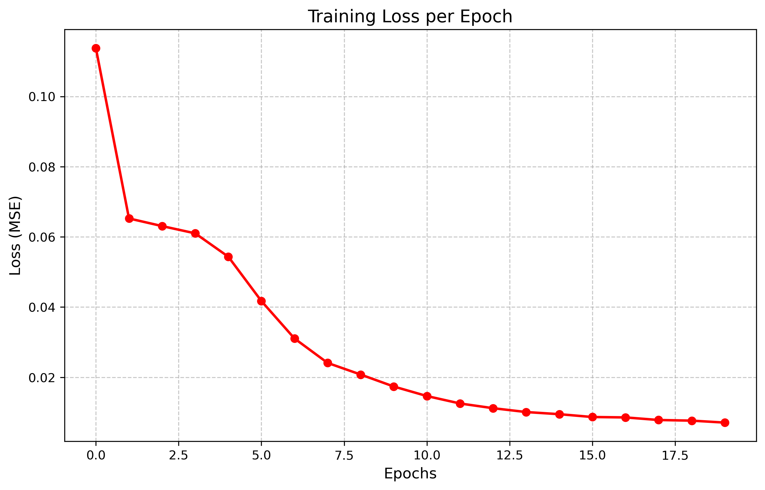
We train the model for 20 epochs. Note that we use MPS device for acceleration
epochs = 20
model.train()
training_loss = []

for epoch in range(epochs):
    running_loss = 0.0
    for batch_i, data in enumerate(train_loader):
        images = data['image'].to(device)
        keypoints = data['keypoints'].to(device)
        keypoints = keypoints.view(keypoints.size(0), -1)

        optimizer.zero_grad()
        output = model(images)
        loss = criterion(output, keypoints)
        loss.backward()
        optimizer.step()

        running_loss += loss.item()

    avg_loss = running_loss/len(train_loader)
    training_loss.append(avg_loss)
    print(f'Epoch {epoch+1}/{epochs}, Loss: {avg_loss:.6f}')

plt.plot(training_loss)
plt.xlabel('Epochs')
plt.ylabel('Loss')
plt.title('Training Loss per Epoch')
plt.show()Epoch 1/20, Loss: 0.104899 Epoch 2/20, Loss: 0.065011 Epoch 3/20, Loss: 0.063819 Epoch 4/20, Loss: 0.060102 Epoch 5/20, Loss: 0.055546 Epoch 6/20, Loss: 0.041323 Epoch 7/20, Loss: 0.030074 Epoch 8/20, Loss: 0.023728 Epoch 9/20, Loss: 0.018558 Epoch 10/20, Loss: 0.015686 Epoch 11/20, Loss: 0.013594 Epoch 12/20, Loss: 0.011677 Epoch 13/20, Loss: 0.010104 Epoch 14/20, Loss: 0.009324 Epoch 15/20, Loss: 0.008212 Epoch 16/20, Loss: 0.007766 Epoch 17/20, Loss: 0.007421 Epoch 18/20, Loss: 0.006695 Epoch 19/20, Loss: 0.006575 Epoch 20/20, Loss: 0.006257
Visualizing the Results of the Model
Finally, we can visualize the prediction of our model on test set faces
test_dataset = FacialKeypointsDataset(root_dir='data/test/', csv_file='data/test_frames_keypoints.csv', transform=data_transform)
test_loader = DataLoader(test_dataset, batch_size=1, shuffle=True)

model.eval()
with torch.no_state_dict if hasattr(torch, 'no_state_dict') else torch.no_grad():
    for i, data in enumerate(test_loader):
        if i >= 2:
            break
        image = data['image'].to(device)
        output = model(image)
        output = output.view(68, 2).cpu().numpy()
        output = output * 50.0 + 100.0

        plt.figure(figsize=(5,5))
        img = image.cpu().squeeze().numpy()
        plt.imshow(img, cmap='gray')
        plt.scatter(output[:, 0], output[:, 1], s=10, marker='.', c='m')
        plt.title(f'Sample {i+1}')
        plt.show()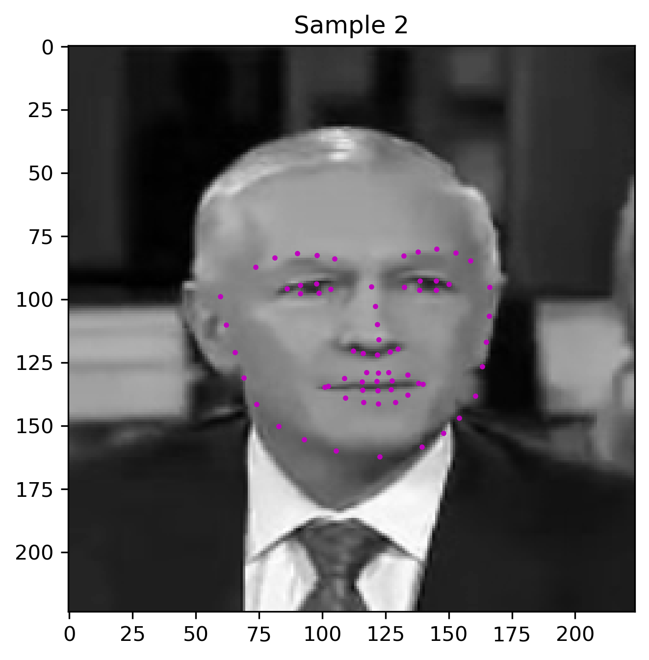
Generating a Grid of Results
Finally, we can generate a grid of results to visualize the model's predictions on a batch of test images
test_dataset = FacialKeypointsDataset(root_dir='data/test/', csv_file='data/test_frames_keypoints.csv', transform=data_transform)
test_loader = DataLoader(test_dataset, batch_size=1, shuffle=True)

# For color images, we need a dataset that only Rescales
color_transform = transforms.Compose([Rescale(224)])
test_dataset_color = FacialKeypointsDataset(root_dir='data/test/', csv_file='data/test_frames_keypoints.csv', transform=color_transform)

# For model input, we need the standard transform
test_dataset_model = FacialKeypointsDataset(root_dir='data/test/', csv_file='data/test_frames_keypoints.csv', transform=data_transform)

model.eval()
fig, axes = plt.subplots(2, 2, figsize=(12, 12))
axes = axes.flatten()

indices = [34, 61, 7, 15] # Just picking some diverse indices

with torch.no_grad():
    for i, idx in enumerate(indices):
        # Get color image
        color_sample = test_dataset_color[idx]
        color_img = color_sample['image']

        # Get model prediction
        model_sample = test_dataset_model[idx]
        image_tensor = model_sample['image'].to(device).unsqueeze(0)
        output = model(image_tensor)
        output = output.view(68, 2).cpu().numpy()
        output = output * 50.0 + 100.0 # De-normalize

        # Plot
        axes[i].imshow(color_img)
        axes[i].scatter(output[:, 0], output[:, 1], s=20, marker='.', c='m')
        axes[i].set_title(f"Sample Index {idx}", fontsize=14)
        axes[i].axis('off')

plt.tight_layout()
plt.show()