Part 1: Building a 68-Facial Keypoint Detection with PyTorch
Facial Keypoint Detection is a crucial task for facial recognition software applications. Facial Keypoint Detection maps human facial features such as the left and right eye, nose, upper and lower lip, and jawline into recognized key points. These key points can then be trained to recognize the presence of a face in an image or video.

In this notebook, I will implement a 68-Facial Keypoint detection project that is available as part of the Udacity Computer Vision Project.
1. Facial Keypoints Dataset
The dataset for this notebook is available here: Udacity Facial Key Point Detection Dataset
Download the dataset
To begin, the following code implements the download and extraction of the dataset into a local folder named "data."
import wget

data_url = 'https://s3.amazonaws.com/video.udacity-data.com/topher/2018/May/5aea1b91_train-test-data/train-test-data.zip'
wget.download(data_url)'train-test-data.zip'
import zipfile

with zipfile.ZipFile('train-test-data.zip', 'r') as zip_file:
    zip_file.extractall('data')
!ls data test training test_frames_keypoints.csv training_frames_keypoints.csv
The facial image dataset has been successfully extracted and loaded into the data folder. The following Unix script can be used to count the number of files at the data folder level.
!find data -type f | cut -d/ -f2 | sort -R | uniq -c3462 training 2308 test 1 training_frames_keypoints.csv 1 test_frames_keypoints.csv
Notice that there are 3462 training images and 2308 test images in the dataset. Additionally, each image file is associated with a corresponding CSV file containing the annotated keypoints.
Understanding the Frame Keypoints CSV files
The "frame_keypoints" CSV files for both the test and train datasets contain the labeled dataset of images along with their respective 68-point facial keypoint detections. These files provide a mapping between each image and the corresponding 68 facial keypoints that have been annotated. To explore and analyze this mapping, let's focus on the training dataset.
import pandas as pd

# Reading and Processing the frames keypoint csv file
train_keypoints = pd.read_csv('data/training_frames_keypoints.csv')
train_keypoints.head()| Unnamed: 0 | 0 | 1 | 2 | 3 | 4 | 5 | 6 | 7 | 8 | ... | 126 | 127 | 128 | 129 | 130 | 131 | 132 | 133 | 134 | 135 | |
|---|---|---|---|---|---|---|---|---|---|---|---|---|---|---|---|---|---|---|---|---|---|
| 0 | Luis_Fonsi_21.jpg | 45.0 | 98.0 | 47.0 | 106.0 | 49.0 | 110.0 | 53.0 | 119.0 | 56.0 | ... | 83.0 | 119.0 | 90.0 | 117.0 | 83.0 | 119.0 | 81.0 | 122.0 | 77.0 | 122.0 |
| 1 | Lincoln_Chafee_52.jpg | 41.0 | 83.0 | 43.0 | 91.0 | 45.0 | 100.0 | 47.0 | 108.0 | 51.0 | ... | 85.0 | 122.0 | 94.0 | 120.0 | 85.0 | 122.0 | 83.0 | 122.0 | 79.0 | 122.0 |
| 2 | Valerie_Harper_30.jpg | 56.0 | 69.0 | 56.0 | 77.0 | 56.0 | 86.0 | 56.0 | 94.0 | 58.0 | ... | 79.0 | 105.0 | 86.0 | 108.0 | 77.0 | 105.0 | 75.0 | 105.0 | 73.0 | 105.0 |
| 3 | Angelo_Reyes_22.jpg | 61.0 | 80.0 | 58.0 | 95.0 | 58.0 | 108.0 | 58.0 | 120.0 | 58.0 | ... | 98.0 | 136.0 | 107.0 | 139.0 | 95.0 | 139.0 | 91.0 | 139.0 | 85.0 | 136.0 |
| 4 | Kristen_Breitweiser_11.jpg | 58.0 | 94.0 | 58.0 | 104.0 | 60.0 | 113.0 | 62.0 | 121.0 | 67.0 | ... | 92.0 | 117.0 | 103.0 | 118.0 | 92.0 | 120.0 | 88.0 | 122.0 | 84.0 | 122.0 |
5 rows × 137 columns
It's important to note the following points:
- 1. Each row in the "frame_keypoints" CSV files corresponds to one image and contains 68 associated key facial points.
- 2. The facial points are represented in a coordinate system $(x, y)$.
Visualizing Sample Image with Facial Keypoints
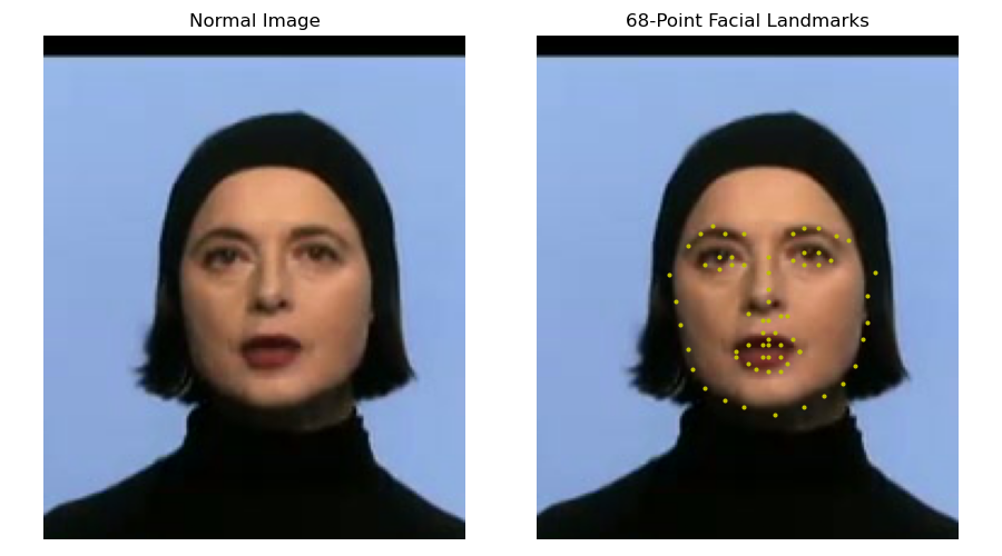
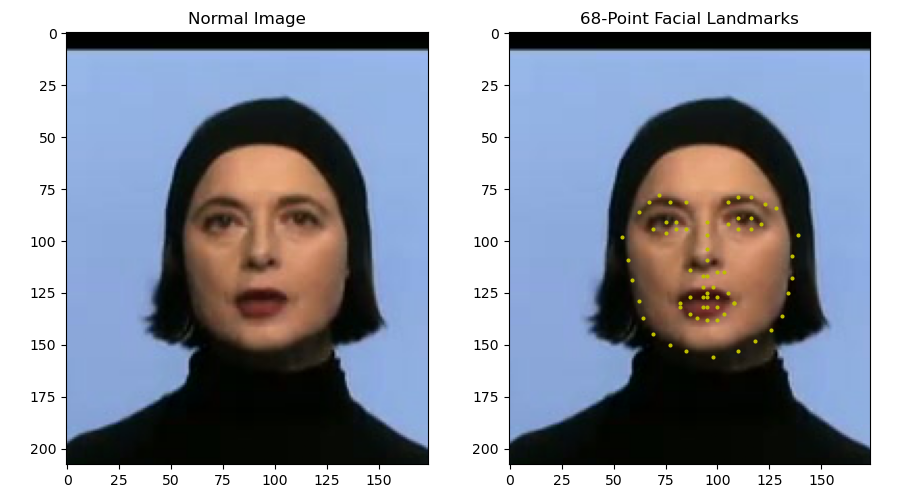
Below is an example code that demonstrates how to map a face to its facial keypoints and visualize the result.
import os
import cv2
import numpy as np
import matplotlib.pyplot as plt
import matplotlib.image as mpimg

%matplotlib inline
%config InlineBackend.figure_format = 'retina'
index = 57
img_name = train_keypoints.iloc[index, 0]
img_keypoints = train_keypoints.iloc[index, 1:].to_numpy()
img_keypoints = img_keypoints.astype('float').reshape(-1, 2)
img = mpimg.imread( os.path.join( 'data', 'training', img_name))
fig, ax = plt.subplots(1, 2, figsize=(9,5))
ax[0].imshow(img)
ax[0].set_title("Normal Image")
ax[1].imshow(img)
ax[1].scatter(img_keypoints[:, 0], img_keypoints[:, 1], s=15, marker='.', c='y' )
ax[1].set_title(f"68-Point Facial Landmarks")

2. Creating PyTorch Dataset Class for Facial Keypoint Detection
Creating a PyTorch Dataset Class for Facial Keypoint Detection is a crucial step in preparing the data for model training. The dataset class will help in handling the images and their corresponding facial keypoints efficiently.
from torch.utils.data import Dataset, DataLoader

class FacialKeypointsDataset(Dataset):

    def __init__(self, root_dir, csv_file, transform=None) -> None:
        self.root_dir = root_dir
        self.keypoints = pd.read_csv(csv_file)
        self.transform = transform

    def __len__(self):
        return len(self.keypoints)


    def __getitem__(self, index):
        image_name = os.path.join(self.root_dir, self.keypoints.iloc[index, 0])
        image = mpimg.imread(image_name)

        # Removing Alpha Channel if it exists
        if image.shape[2] == 4:
            image = image[:, :, 0:3]

        keypoints = self.keypoints.iloc[index, 1:].to_numpy()
        keypoints = keypoints.astype('float').reshape(-1, 2)
        sample = { 'image': image, 'keypoints': keypoints }

        if self.transform:
            sample = self.transform(sample)

        sample = { 'image': image, 'keypoints': keypoints }
        return sample
faces_dataset = FacialKeypointsDataset(root_dir='data/training/', csv_file='data/training_frames_keypoints.csv')
len(faces_dataset)3462
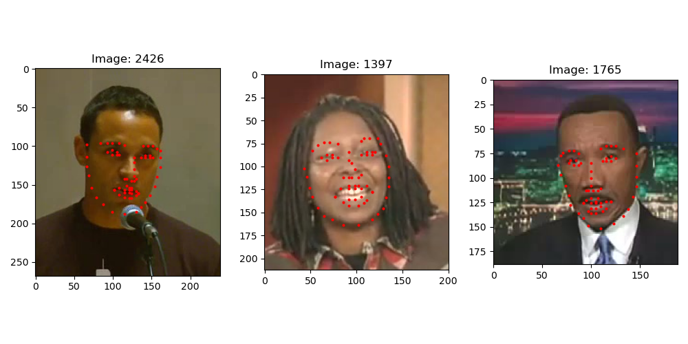
With the dataset setup, we can retrieve samples from the dataset using indexes and use the view_facial_keypoints() function below to render the images. The example below renders a random sample of three images from the dataset and displays those images.
# function to view the image
def view_facial_keypoints(img, keypoints):
    plt.imshow(img)
    plt.scatter(keypoints[:, 0], keypoints[:, 1], s=15, marker='.', c='r')


fig = plt.figure(figsize=(10,5))

for i in range(3):

    idx = np.random.randint(len(faces_dataset))
    sample_image = faces_dataset[idx]

    ax = plt.subplot(1, 3, i+1)
    ax.set_title(f'Image: {idx}')

    view_facial_keypoints(sample_image['image'], sample_image['keypoints'])

3. Image Transforms and Data Augmentation
In the sample images above, it is noticeable that each image has varying dimensions. To handle inputs into a Convolutionary Neural Network, we need to resize all images to a single dimension. Additionally, we will need to normalize and augment the dataset to develop a robust model.
The transforms below implement the following steps:
- 1. Normalize: Scale pixel intensities to values between zero and 1.
- 2. Rescale: Scales the images into equal height and width for all images.
- 3. RandomCrop: Allows for random cropping of the image to introduce complexity within the dataset.
import torch
from torchvision import transforms, utils


class Normalize:

    def __call__(self, sample):
        image, keypoints = sample['image'], sample['keypoints']

        image_copy = np.copy(image)
        keypoints_copy = np.copy(keypoints)

        # converts to gray scale before normalization
        image_copy = cv2.cvtColor( image, cv2.COLOR_RGB2GRAY )
        image_copy = image_copy/255.0

        # mean = 100, sqrt = 50,
        keypoints_copy = (keypoints_copy - 100)/50

        return {'image': image_copy,'keypoints' : keypoints}


class Rescale:

    def __init__(self, outputsize) -> None:
        assert isinstance(outputsize, (int, tuple))
        self.outputsize=outputsize


    def __call__(self, sample):
        image, keypoints = sample['image'], sample['keypoints']

        h, w = image.shape[:2]
        if isinstance(self.outputsize, int):
            if h > w:
                new_h, new_w = self.outputsize * h/w, self.outputsize

            else:
                new_h, new_w = self.outputsize, self.outputsize * w/h

        else:
            new_h, new_w = self.outputsize


        new_h, new_w = int(new_h), int(new_w)
        img = cv2.resize(image, (new_w, new_h))

        keypoints = keypoints * [ new_w/w, new_h/h ]

        return { 'image': img, 'keypoints': keypoints }


class RandomCrop:

    def __init__(self, outputsize):
        assert isinstance(outputsize, (int, tuple))
        #if type is integer then it will be used for both width and height

        if isinstance(outputsize, int):
            self.outputsize = (outputsize, outputsize)
        else:
            assert len(outputsize) == 2
            self.outputsize = outputsize


    def __call__(self, sample):
        image, keypoints = sample['image'], sample['keypoints']
        h, w = image.shape[:2]
        new_h, new_w = self.outputsize

        top = np.random.randint(0, h - new_h)
        left = np.random.randint(0, w - new_w)

        image = image[ top: top + new_h, left: left + new_w ]
        keypoints = keypoints - [left, top]

        return {'image': image, 'keypoints': keypoints}


class ToTensor:

    def __call__(self, sample):
        image, keypoints = sample['image'], sample['keypoints']

        if len(image.shape) == 2:
            image = image.reshape(image.shape[0], image.shape[1], 1)


        # swap color axis because
        # numpy image: H x W x C
        # torch image: C X H X W
        image = image.transpose((2, 0, 1))

        return {'image': torch.from_numpy(image), 'keypoints': torch.from_numpy(keypoints) }
Combining the Classes into a Transform Compose
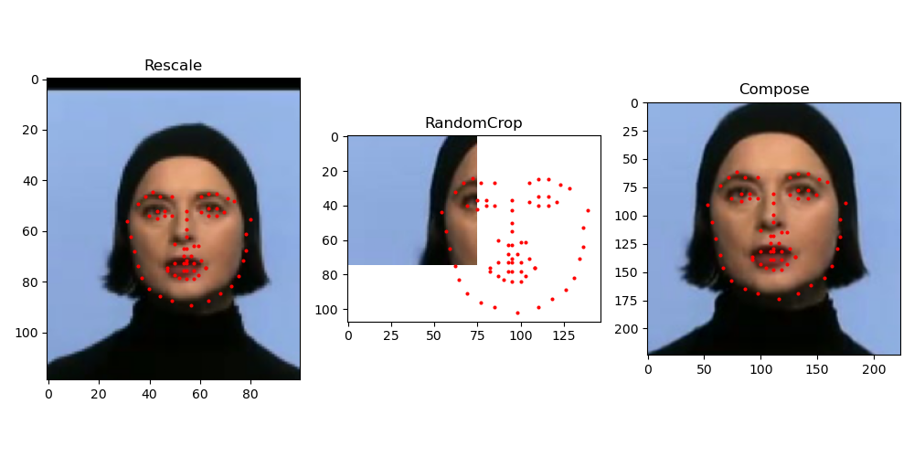
Pytorch offers transform.Compose() method which combines various image transformations. The code below demonstrates both individual and the combination of the transforms.
rescale = Rescale(100) # rescales images to 100 pixels
crop = RandomCrop(75)  # crop 75 pixels at random
composed = transforms.Compose( [ Rescale(250), RandomCrop(224) ] )


# sampling image 57
sample_image = faces_dataset[57]


fig = plt.figure(figsize=(15, 5))

for i,transform in enumerate( [ rescale, crop, composed ] ):
    trasnformed_sample = transform(sample_image)

    ax = plt.subplot(1, 3, i + 1)
    plt.tight_layout()
    ax.set_title(type(transform).__name__ )
    view_facial_keypoints(trasnformed_sample['image'], trasnformed_sample['keypoints'])
Implementing Transforms on the Dataset
Now that we have demonstrated the transforms, we can implement the compose as part of the dataset class. This will ensure all images are processed used the same sequency of transforms.
image_transforms = transforms.Compose( [ Rescale(250), RandomCrop(224), Normalize(), ToTensor() ])

transformed_dataset = FacialKeypointsDataset( csv_file='data/training_frames_keypoints.csv',
                                                root_dir='data/training/',
transform=image_transforms )transformed_dataset[57]['image']tensor([[[0.0028, 0.0028, 0.0028, ..., 0.0027, 0.0027, 0.0027],
[0.0028, 0.0028, 0.0028, ..., 0.0027, 0.0027, 0.0027],
[0.0028, 0.0028, 0.0028, ..., 0.0027, 0.0027, 0.0027],
...,
[0.0025, 0.0025, 0.0025, ..., 0.0026, 0.0026, 0.0026],
[0.0025, 0.0025, 0.0025, ..., 0.0026, 0.0026, 0.0026],
[0.0025, 0.0025, 0.0025, ..., 0.0026, 0.0026, 0.0026]]])This completes the first section of this note. The second begins with Model Architecture and completes training and evaluation of the model