Modeling Diminishing Returns Regression with Python: Cost vs. Revenue Case
In economics, the concept of diminishing returns pertains to the correlation between the cost and overall output of a product or service. It observes that assuming all factors remain the same, an increase in unit production cost leads to a decrease in the marginal yield of the entire production. In other words, there comes a juncture during the production process where an extra investment, such as hiring another employee, results in a lower output per unit cost.
Working as a data scientist in digital marketing, a significant amount of my time is spent on building cost-to-revenue optimization models for clients who often have a single budget across a diverse set of product verticals and categories. The objective is to find the optimal spend allocation which first begins with modeling diminishing returns by vertical
This note looks at a singular case of building a diminishing returns model on cost to revene data
Weekly Sales and Revenue Data
This note utilizes weekly cost and revenue data to model a diminishing returns process. The data has been pre-processed to eliminate outliers and was scaled to facilitate the analysis.
import numpy as np
import pandas as pd
import matplotlib.pyplot as plt

%matplotlib inline
%config InlineBackend.figure_format = 'retina'
data = pd.read_csv('weekly_spend_to_revenue_data.csv')
data.head()| cost | revene | |
|---|---|---|
| 0 | 208 | 439.580708 |
| 1 | 293 | 439.898090 |
| 2 | 196 | 439.574561 |
| 3 | 185 | 439.339671 |
| 4 | 267 | 439.815404 |
Visualizing the data
To see the full picture on the data, I apply a scatter plot visualization to determine if the diminishing returns trend exists
plt.figure(figsize=(7,5))
plt.title('Scatter Plot: Weekly Cost vs Revenue', fontsize=8)
plt.scatter(data.cost, data.revenue, marker='.', s=10)
plt.xlabel('weekly_cost', fontsize=8)
plt.ylabel('weekly_revenue', fontsize=8)
plt.xticks(fontsize=8)
plt.yticks(fontsize=8)
plt.tight_layout()
plt.show()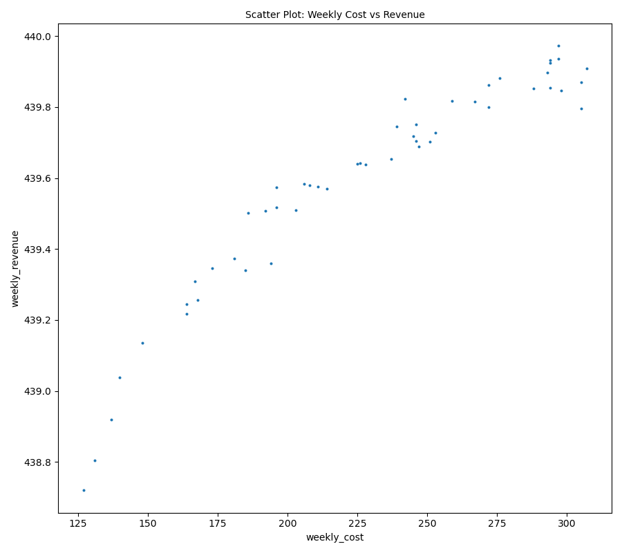
Modeling Diminishing Returns Functions
Several mathematical functions can be used to model the diminishing returns relationship. On this note, I focus on two key functions:
- 1. Power Function
- 2. Michaelis-Menten Function
1. Power Function
The power function can be used to model non-linear relationships with a lot of flexibility due to the beta parameter. Mathematically, it is represented as:
$$ f(x) = \alpha * x^{\beta} $$
where:
$\alpha$: is a scalar parameter for scaling the power function
$\beta$: define the non-linear form with varying values
Below are a few examples of the power function at different $\beta$ levels.
2. Michaelis-Menten Function
Michaelis-Menten function that is finds its root in biology looking at Enzyme reaction. The functional form can be used for modeling diminishing returns with constraints on parameters. The mathematical definition of the function is:
$$ f(x) = \frac {\alpha * x } { 1 + \beta * x} $$
Below are a few examples of the power function at different $\beta$ levels.
Fitting Diminishing Returns with curve_fit()
To fit the model on the data, we first define Python functions that take the form of diminishing returns functions above.
def michaelis_menten(x, alpha, beta):
    return (alpha * x)/(1 + beta*x)


def power_function(x, alpha, beta):
    return alpha * x ** beta


dim_returns_funcs = { 'michaelis_menten': michaelis_menten, 'power_function':  power_function }
curve_fit() method
The curve_fit takes in as arguments, the mathematical function to model and it's x and y values. It returns a number of parameters all which are available here
For this case, I am interested in the point estimates of $\alpha$ and $\beta$ params.
from scipy.optimize import curve_fit

# Iterative Fitting the Model
params = {}
for name, func in dim_returns_funcs.items():

    # fit the curve and return parameters
    model_params = curve_fit(func, data.cost, data.revenue)[0]
params[name] = model_paramsparams{'michaelis_menten': array([793.72074501, 1.80094172]),
'power_function': array([4.33199306e+02, 2.71103403e-03])}Running Predictions
With the alpha and beta values return, we can make predictions and see how our models fit the actual data.
In order to plot line chats, we need to create an ordered array the size of the data with a min and max of the cost array
ordered_xvalues = np.linspace( data.cost.min(), data.cost.max(), len(data) )
data['ordered_xvalues'] = ordered_xvalues

for name, coeff in params.items():
    # predictions against the data
    data[name] = dim_returns_funcs[name]( data.cost , coeff[0], coeff[1])
    # for line plot
data[name + '_ordered'] = dim_returns_funcs[name](ordered_xvalues, coeff[0], coeff[1] )| cost | revene | ordered_xvalues | michaelis_menten | michaelis_menten_ordered | power_function | power_function_ordered | |
|---|---|---|---|---|---|---|---|
| 0 | 208 | 439.580708 | 127.000000 | 439.551988 | 438.806854 | 439.513380 | 439.513380 |
| 1 | 293 | 439.898090 | 130.673469 | 439.891751 | 438.860560 | 439.921831 | 438.959860 |
| 2 | 196 | 439.574561 | 134.346939 | 439.480349 | 438.911340 | 439.442581 | 438.992854 |
| 3 | 185 | 439.339671 | 138.020408 | 439.406542 | 438.959428 | 439.373776 | 439.024960 |
| 4 | 267 | 439.815404 | 141.693878 | 439.810741 | 439.005033 | 439.811020 | 439.056224 |
fig = plt.figure(figsize=(7,6))
plt.scatter(data.cost, data.revenue, marker='.', s=11, label='actual_revenue')
plt.plot(data.ordered_xvalues, data.michaelis_menten_ordered,  '-.', color='seagreen', label='Michaelis Menten Prediction')
plt.plot(data.ordered_xvalues, data.power_function_ordered, '-.', color='orange',  label='Power Funtion Prediction')
plt.title('Actual vs. Predictions', fontsize=8)
plt.xlabel('weekly_cost', fontsize=8)
plt.ylabel('weekly_revenue', fontsize=8)
plt.legend(fontsize=6)
plt.tight_layout()
plt.show()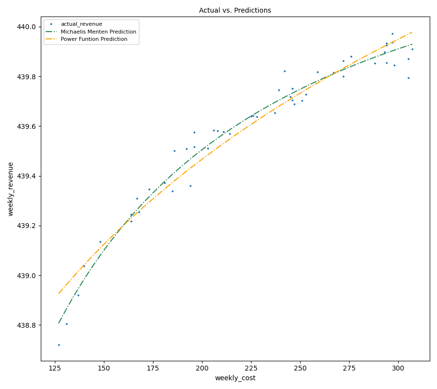
Model Fit Assessment
Visually, both models seem to fit the data quite well, with Michaelis-Menten showing a slightly better fit. To numerically quantify the goodness of fit of each model, a simple $R^2$ assessment will be utilized.
def r_squared(actual, prediction):
    ssr = np.sum( (prediction - np.mean(actual))**2  )
    sst = np.sum( (actual - np.mean(actual)) ** 2 )
    return round( 100* ssr/sst, 3)
michaelis_menten_rsquared = r_squared( data.revenue, data.michaelis_menten )
power_function_rsquared = r_squared(data.revenue, data.power_function)
michaelis_menten_rsquared, power_function_rsquared(97.28, 94.56)
Both fits perform really well in modeling the diminishing returns data with Michaelis-Menten edging over the Power function.