Masking
Masking is a technique used in computer vision that can achieve results similar to chroma keying in video and filmmaking. While chroma keying uses green screens during filming to replace the green background with another image or footage during post-production, masking targets pre-defined pixel intensity ranges and replaces those pixels falling into the range with white and those out of the range with black.
For instance, if the background in an image is green or blue, we can use masking to select a range of blue hues, and all areas of blue within the image will be highlighted while non-blue areas will be turned to zero. This technique can be used to separate objects from their background, remove unwanted elements from images, or create custom image filters. In short, masking allows us to manipulate and modify images by selecting specific ranges of pixel intensity.
This example demonstrates masking of the following process.
Masking with OpenCV
The OpenCV inRange() can be used to create a mask of an image. It works by targeting a range of pixel intensity provided and returns a mask. Let's see an example:
import numpy as np
import cv2
import matplotlib.pyplot as plt

%matplotlib inline
%config InlineBackend.figure_format = 'retina'
tangerine = cv2.imread('../images/tangerine.jpg')
tangerine = cv2.cvtColor(tangerine, cv2.COLOR_BGR2RGB)
plt.imshow(tangerine)
plt.axis('off')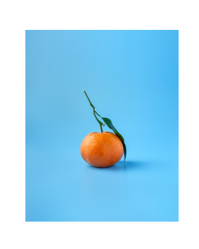
Creating a Mask
To create a mask, it is necessary to define a lower and upper bound for the color range being targeted. In the case of blue, finding the appropriate color range can be challenging and may require experimentation.
One approach to identifying the appropriate range is to loop through the image and find all RGB combinations where the maximum pixel intensity falls on the blue channel. Using this method, the lower and upper bounds can be determined to define the range of blue being targeted for masking.
In this example, the process of looping through the image to identify the appropriate bounds resulted in the following values being selected as the lower and upper bounds for the blue color range.
lower_bound = np.array([0, 90, 140])
upper_bound = np.array([205, 245, 255])
mask = cv2.inRange(tangerine, lower_bound, upper_bound)
plt.imshow(mask, cmap='gray')
plt.axis('off')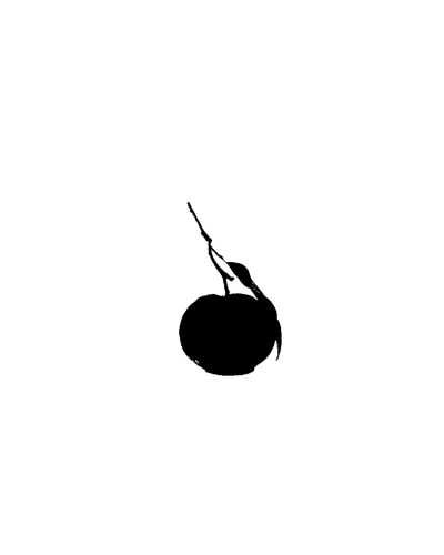
Notice that with the mask, all the blue pixels are turned on (set to white) while the non-blue pixels are set to black.
Now that we have a mask, let's use it to super-impose another image.
space = cv2.imread('../images/space.jpg')
space = cv2.cvtColor(space, cv2.COLOR_BGR2RGB)

# Resizing space to tangerize shape
space = cv2.resize(space, tangerine.shape[:2][::-1], interpolation=cv2.INTER_AREA )

plt.imshow(space)
plt.axis('off')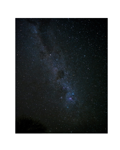
To super-impose, we implement three steps:
- 1. Replace pixels on the original image that correspond to white pixels on the mask to zero.
tangerine[ mask != 0] = [0, 0, 0]

plt.imshow(tangerine)
plt.axis('off')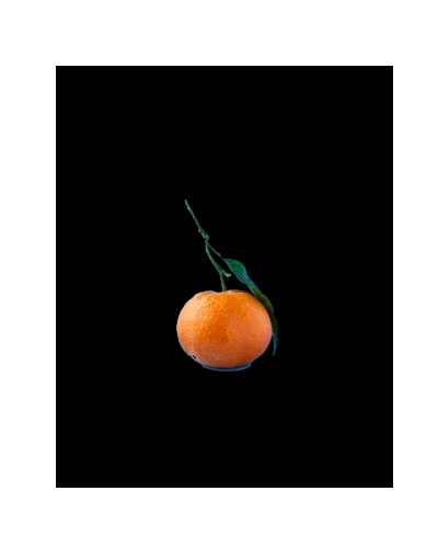
- 2. Replace pixels on the new/background image that correspond to black pixels on the mask to zero
space[ mask == 0] = [0, 0, 0]

plt.imshow(space)
plt.axis('off')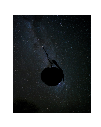
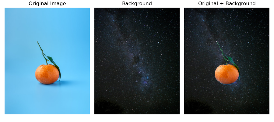
- 3. Add the two images together.
tangerine_in_space = tangerine + space

plt.imshow(tangerine_in_space)
plt.axis('off')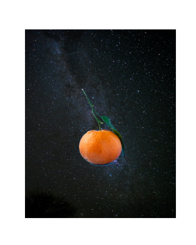
Masking, like many computer vision techniques tend to work well with normalized images. Applying a GaussianBlur, for example, can help with clearing spots of blue that may be on the tangerine in the image above.