Kernel Convolutions with OpenCV
In the previous note, we discussed the theoretical implementations of Kernel Convolutions. This short note demonstrates kernel convolutions with OpenCV.
Convolution with OpenCV work in much the same way as convolution with ndimage. We will use an example of a butterfly image and apply the following kernels.
$$ kernel_1= \begin{pmatrix} 1 & 1 & 1 \\ 1 & 1 & 1 \\ 1 & 1 & 1 \end{pmatrix}, kernel_2 = 1/9 * \begin{pmatrix} 1 & 1 & 1 \\ 1 & 1 & 1 \\ 1 & 1 & 1 \end{pmatrix}, kernel_3 = \begin{pmatrix} -1 & -1 & -1 \\ -1 & 8 & -1 \\ -1 & -1 & -1 \end{pmatrix}$$
Implementation in OpenCV
import cv2
import numpy as np
import matplotlib.pyplot as plt

%matplotlib inline
%config InlineBackend.figure_format = 'retina'
img = cv2.imread('butterfly.jpg')
img = cv2.cvtColor(img, cv2.COLOR_BGR2RGB)
# image show
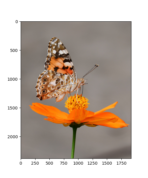
plt.imshow(img)
Defining Kernels
kernel_1 = np.ones(shape=(3,3))
kernel_2 = 1/9*(kernel_1)

kernel_3 =  -1*(np.ones(shape=(3,3)))
kernel_3[1,1] = 8

kernel_1, kernel_2, kernel_3
OUTPUT
(array([[1., 1., 1.],
    [1., 1., 1.],
    [1., 1., 1.]]),
array([[0.11111111, 0.11111111, 0.11111111],
    [0.11111111, 0.11111111, 0.11111111],
    [0.11111111, 0.11111111, 0.11111111]]),
array([[-1., -1., -1.],
    [-1.,  8., -1.],
    [-1., -1., -1.]]))
Convolution Implementation
To implement a convolution with OpenCV, we use the method cv2.filter2D(). The method takes the following arguments:
- 1. src: input image we wish to convolve
- 2. depth: destination depth (). In this case, we use -1 to signify the source image depth is to be used for the destination image
- 3. kernel: the kernel matrix
convolved_k1 = cv2.filter2D(img, -1, kernel_1)
convolved_k2 = cv2.filter2D(img, -1, kernel_2)
convolved_k3 = cv2.filter2D(img, -1, kernel_3)
Visualizing the convolution outcome
fig = plt.figure(figsize=(8,10))

fig.add_subplot(221)
plt.imshow(img)
plt.title('Original Image')

fig.add_subplot(222)
plt.imshow(convolved_k1)
plt.title('Convolution K1')

fig.add_subplot(223)
plt.imshow(convolved_k2)
plt.title('Convolution K2')


fig.add_subplot(224)
plt.imshow(convolved_k3)
plt.title('Convolution K3')

plt.tight_layout()
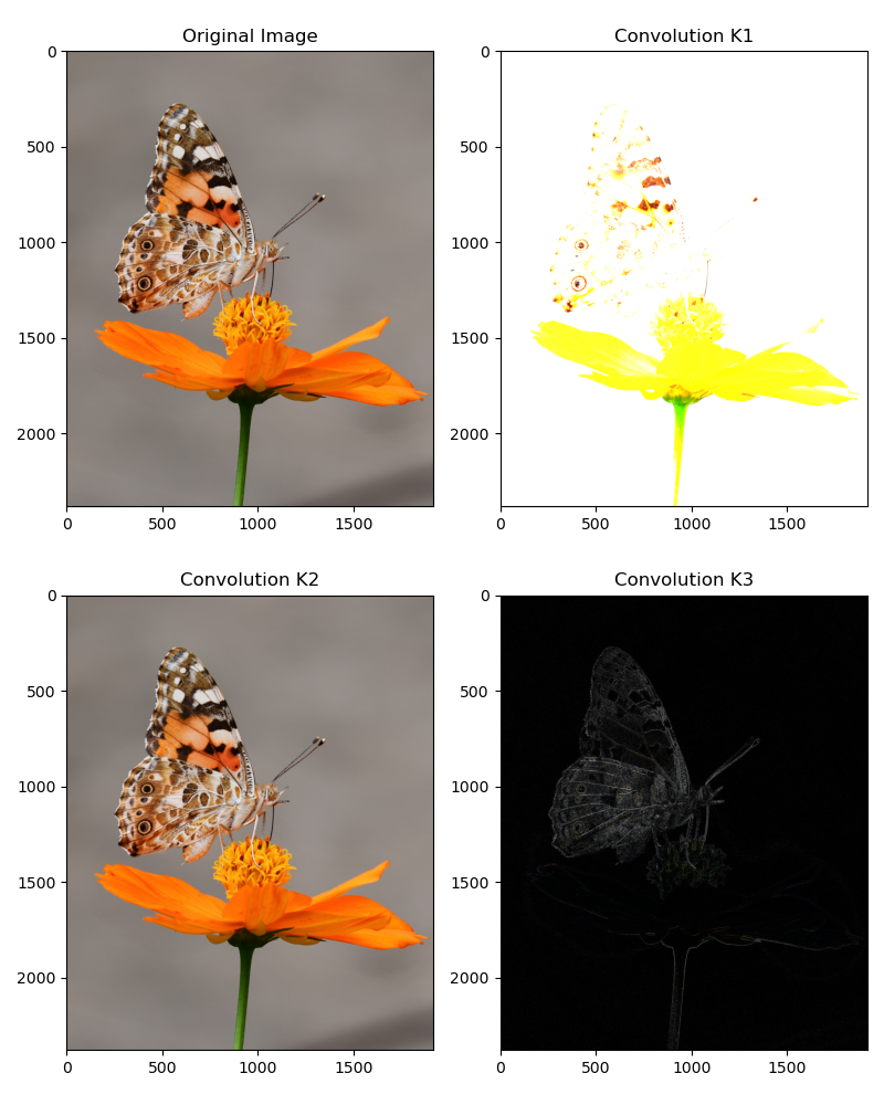
Notice that a couple of useful things:
- 1. The first kernel simply resulted in the sum of neighbor pixels to the center pixel. This has the effect of brightening the image overall.
- 2. The second kernel takes the weighted sum of the neighbor pixels and averages them. This often has the effect of blurring the image.
- 3. The third kernel which is often used for enhancing edges magnifies the center pixel with a high weight while reducing the neighboring pixels with a negative weight.