Gradient Descent Algorigthm
For a number of years, I used statistical enterprise software like Minitab and Stata for Econometrics work particularly in modeling Regression and Time Series forecasting. These tools have abstracted the technical implementation and algorithms that I barely need to go beyond the UI to generate a well performing model.
Even as I moved to Python and R, many of the packages have the same abstractions, albeit not quite at the UI level. For example, you can easily fit a model by calling model.fit() in python. These abstractions have reduced the barier of entry into ML and Data Science, even for those that are mathematically inclined but perhaps less saving with programming.
It was until I began working with deep learning tools like Pytorch which demand the user to outline a training routine, that I discovered the necessity to learn how to implement optimization algorithms and make parameter choices that lead to the best results. This was also the first time I realized that the closed-form solutions I learned in my Econometrics and Statistics courses are not nearly as useful in practice.
Parameters Estimation of the Simple Linear Regression Problem
Simple linear regression is a great introductory example of statistical modeling, as it involves estimating only two parameters and introduces important concepts such as the measure of fit, residuals, and cost functions, which can easily become convoluted with additional parameters.
Recall the linear model:
$$ y = \beta_0 + \beta_1*x + \epsilon$$
The process of estimating $\beta_0$ and $\beta_1$ stats with formulating a cost function.
$$ residual = y - \widehat{y} $$
where $y$ are actual values and $\widehat{y}$ are predicted values.
But since our goal is to reduce the overall difference between $y$ and $\widehat{y}$, we reformulate the loss function into RSS (Residual Sum of Squares).
This is mathematically represented as:
$$ RSS = \sum_{n=i}^{N} ({y_i - \widehat{y_i}})^2$$
This is the same as:
$$ \sum_{n=i}^{N} (y_i - (\widehat{\beta_0} + \widehat{\beta_1}*x))^2 = \sum_{n=i}^{N} (\epsilon_i)^2$$
So now, there is an objective function. The goal is to minimize the function which means determining the values of $\beta_0$ and $\beta_1$ that achieve that.
$$\min_{\beta_0, \beta_1} \sum_{n=i}^{N} (y_i - (\widehat{\beta_0} + \widehat{\beta_1}*x))^2$$
Closed Form Solution
Here is where some calculus comes in. To determine the values of $\beta_0$ and $\beta_1$, we implement partial derivatives on the cost function with respect to $\beta_0$ and $\beta_1$.
Case 1: $\beta_0$
$$ \frac{\partial RSS(\beta_0, \beta_1)} {\partial \beta_0} = \sum 2[y_i - (\widehat{\beta_0} + \widehat{\beta_1} x_i)](-1) $$
Equate the partial to Zero:
$$ 0 = -2 \sum y_i - \sum \widehat{\beta_0} - \sum \widehat{\beta_1} x_1 $$
$$\sum \widehat{\beta_0} = \sum y_i - \widehat{\beta_1} \sum x_i$$
Recall, the sum of a constant is equal to constant multiplied by n:
$$n\widehat{\beta_0} = \sum y_i - \widehat{\beta_1} \sum x_i$$
$$\widehat{\beta_0} = \frac {\sum y_i}{n} - \frac{ \widehat{\beta_1} \sum x_i} {n}$$
Therefore: $$\widehat{\beta_0} = \bar y - \widehat{\beta_1}*\bar x $$
Case 2: $\beta_1$
$$ \frac{\partial RSS(\beta_0, \beta_1)} {\partial \beta_0} = \sum 2[y_i - (\widehat{\beta_0} + \widehat{\beta_1} x_i)](-x_i)$$
Equate the partial to Zero:
$$ 0 = -2 \sum y_i x_i - \sum \widehat{\beta_0} x_i - \sum \widehat{\beta_1} x_1^2$$
$$ 0 = -2 \sum y_i x_i - \widehat{\beta_0} \sum x_i - \widehat{\beta_1} \sum x_1^2 $$
Substitute $\beta_0$ in the equation:
$$ 0 = -2 \sum y_i x_i - (\bar y + \widehat{\beta_1} \bar x) \sum x_i - \widehat{\beta_1} \sum x_1^2 $$
$$ 0 = \sum y_i x_i - \bar y \sum x_i + \widehat{\beta_1} \bar x \sum x_i - \widehat{\beta_1} \sum x_1^2 $$
We can simplify the equation using summation rules to:
$$ \widehat {\beta_1} = \frac {\sum x_i y_i - n\bar x^2} {\sum x_i^2 - n\bar x^2} $$
$$ \widehat {\beta_1} = \frac {\sum (x - \bar x) (y - \bar y)} {\sum (x - \bar x)^2} = \frac {Cov(X,Y)}{Var(x)}$$
Implementation in Code
The closed solution can be implemented in Python in the example below.
import numpy as np

class SLRClosedForm:

    def __init__(self, feature, target):
        self.feature = feature
        self.target = target

    def __str__(self):
        return "Simple Linear Regression Class"

    def closed_form_solution(self):
        numerator = np.sum((self.feature - np.mean(self.feature)) * (self.target - np.mean(self.target)))
        denominator = np.sum((self.feature - np.mean(self.feature))**2)
        beta = numerator/denominator
        alpha = np.mean(self.target) - beta*(np.mean(self.feature))
        return alpha, beta

    def residual_sum_squares(self, alpha, beta):
        return np.sum((self.target - (alpha + beta*self.feature))**2)

    def prediction(self, alpha, beta):
        return alpha + beta*self.feature
Gradient Descent Algorithm
In matrix notation, the closed-form solution is given by:
$$ \beta = (H^TH)^{-1}H^Ty$$
where:
$\beta$: vector of all coefficients
$H$: input matrix (matrix of our input variables)
$y$: vector of the target variable
Inverting a matrix is computationally prohibitive, therefore, gradient descent is a much better option. Below is the theoretical solution in a few steps:
- 1. Initialize a vector of our parameters $\beta$ set to Zero
- 2. Define step Size for parameter updating. We can set this as a decaying value
- 3. Implement partial derivative for every parameter in the model
$$\frac {\partial RSS(\beta)}{\beta_i} = -2\sum x_i (y_i - \widehat y(\beta))$$
- 4. Update the parameter at each step. $t$ is the step size
$$\beta_i^{t+1} = \beta_i^{t} - t * \frac {\partial RSS(\beta)}{\beta_i} $$
- 5. Check convergence criteria.
$$\| \nabla RSS(\beta^{t}) \| > \epsilon$$
where:
$\epsilon$: is a predefined tolerance
In Summary
$$ while\ \| \nabla RSS(\beta^{t}) \| > \epsilon: $$
$$ for\ i = 0,1,...,D $$
$$\frac {\partial RSS(\beta)}{\beta_i} = -2\sum x_i (y_i - \widehat y(\beta))$$
$$\beta_i^{t+1} = \beta_i^{t} - t * \frac {\partial RSS(\beta)}{\beta_i}$$
Implementation in Python
The implementation in Python can be seen below.
class SLRGradientDescent:

    def __init__(self, feature, target):
        self.feature = feature
        self.target = target

    def __str__(self):
        return "Simple Linear Regression Class"

    def gradient_parameter(self, tolerance):
        """ Gradient Descent Algorithm """
        self.alpha = 0
        self.beta = 0
        self.count = 0
        self.stepsize = .001

        error = self.target - (self.alpha + self.beta * self.feature)
        magnitude = abs(np.sum(error))
        while magnitude > tolerance:
            """ Updating the Intercept"""
            self.alpha = self.alpha + self.stepsize*np.sum(error)
            self.beta = self.beta + self.stepsize*np.sum(error*self.feature)

            self.count += 1
            error = self.target - (self.alpha + self.beta * self.feature)
            magnitude = abs(np.sum(error))

        print("Total Updates:", self.count)
        return self.alpha, self.beta
Closed Solution and Gradient Descent in Action
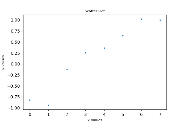
To demonstrate that they both return expected parameters, I'll run both algorithms on a simple linear regression problem. For simplicity, we'll make the dataset very small and predictable.
import numpy as np
import sklearn.datasets as ds
import matplotlib.pyplot as plt

%matplotlib inline
%config InlineBackend.figure_format = 'retina'
x = np.array([0., 1., 2., 3., 4., 5., 6., 7.])
y = np.array([-.82, -.94, -.12, .26, .36, .64, 1.02, 1.])fig = plt.figure(figsize=(6, 4))
plt.scatter(x=x, y=y, marker='o', s=4)
plt.xlabel('x_values', fontsize=8); plt.ylabel('y_values', fontsize=8)
plt.show()
Closed Form Solution
Below is the Closed Form Solution implementation to the sample data
### Closed Form Solution
closed_model = SLRClosedForm(x, y)

alpha, beta = closed_model.closed_form_solution()
closed_solution_y = alpha + beta * x

print('Alpha is {} ,'.format( round(alpha, 2) ),'Beta is {}'.format( round(beta, 2)))Alpha is -0.86 , Beta is 0.3
Gradient Descent Solution
Below is the Gradient Descent Solution implementation to the sample data
### Gradient Descent Solution

gradient_descent = SLRGradientDescent(x, y)
alpha, beta = gradient_descent.gradient_parameter(.0001)
print(alpha, beta)

gradient_descent_y = alpha + beta * x Total Updates: 4300 (-0.863290064203992, 0.2966578678995444)
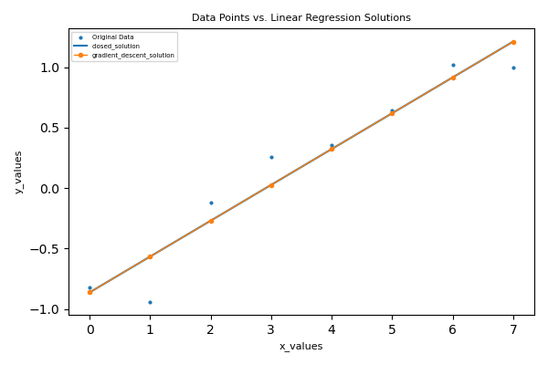
The parameters estimates are nearly the same and we would expect that to reflect in the visualization as well.
fig = plt.figure(figsize=(5, 4))
plt.scatter(x=x, y=y, marker='o', s=4, label='Original Data')
plt.title('Data Points vs. Linear Regression Solutions', fontsize=8)

plt.plot(x, closed_solution_y, label='closed_solution')
plt.plot(x, gradient_descent_y, marker='.', label='gradient_descent_solution', linewidth=1)
plt.xlabel('x_values', fontsize=8);
plt.ylabel('y_values', fontsize=8)

plt.legend(fontsize=5)
plt.tight_layout()