Detecting COVID19 on XRay Images with CNN
Computer vision has revolutionized the healthcare and medical industry by providing powerful tools for the detection and diagnosis of medical conditions and diseases. With the help of computer applications trained to recognize patterns on medical image data, it is now possible to screen and detect medical conditions at scale. One of the many applications of computer vision in this field is the detection of diseases on medical image data such as x-rays.
In this note, we explore the use of Convolutional Neural Networks (CNNs) to develop a classification model capable of predicting COVID-19 cases based on x-ray images. To achieve this, we leverage the COVID-19 x-ray dataset available at https://github.com/ieee8023/covid-chestxray-dataset
COVID DATASET
The COVID dataset used to train the model contains a total of 184 x-ray images. The images are split in the following way.
Train:
$covid: 112$, $Normal: 112$
Validation:
$covid: 30$, $Normal: 30$
For more details on the dataset, see the github link provided.
1. Dataset Prep and Visualization.
The first step is to download, process and visualize the data that we will be using for training. To process the data, we will use torchvision.datasets.ImageFolder() for image manipulation such as resizing, cropping and converting the images into a PyTorch dataset.
An important note here is that the datasets.ImageFolder() class expects a folder structure for which each subfolder represents a class/category and all images in the subfolder are of that class. For example, all covid positive images in the train folder will be in Covid subfolder and normal images will be in the Normal subfolder.
Here is an example of how to structure your image data.
! tree data -ddata
├── Train
│ ├── Covid
│ └── Normal
└── Val
├── Covid
└── Normal
1.1. Importing images into PyTorch Dataset with datasets.ImageFolder()
torchvision's ImageFolder() method is a useful utility class that converts raw images from folders to a dataset object that can interact with PyTorch modules. It takes two arguments: root_folder_path and transforms.
Creating transforms is important because images will need to be resized and converted to tensors before using them for model training.
import torch
import matplotlib.pyplot as plt
from torch.utils.data import DataLoader, Dataset

import torchvision
from torchvision import transforms, datasets

%matplotlib inline
%config InlineBackend.figure_format = 'retina'
For the transform, I implement two sequence of transformations.
- 1. Resize all photos to a 224 x 224 x 3
- 2. Crop Image from the center.
transform = transforms.Compose([ transforms.Resize(224), transforms.CenterCrop(224), transforms.ToTensor()])
train_dataset = datasets.ImageFolder('data/Train/', transform=transform)
The train_dataset is now a PyTorch dataset class. This mean, I can retrive individual image tensors and their class.
train_dataset[-1][0]tensor([[[0.8510, 0.8510, 0.8392, ..., 0.3451, 0.3294, 0.3216],
[0.6863, 0.6784, 0.6706, ..., 0.2588, 0.2431, 0.2353],
[0.5451, 0.5373, 0.5255, ..., 0.2235, 0.2118, 0.2000],
...,
[0.0078, 0.0471, 0.0745, ..., 0.4039, 0.4118, 0.4157],
[0.0039, 0.0471, 0.0745, ..., 0.4235, 0.4275, 0.4314],
[0.0039, 0.0392, 0.0706, ..., 0.4275, 0.4353, 0.4392]],
[[0.8510, 0.8510, 0.8392, ..., 0.3451, 0.3294, 0.3216],
[0.6863, 0.6784, 0.6706, ..., 0.2588, 0.2431, 0.2353],
[0.5451, 0.5373, 0.5255, ..., 0.2235, 0.2118, 0.2000],
...,
[0.0078, 0.0471, 0.0745, ..., 0.4039, 0.4118, 0.4157],
[0.0039, 0.0471, 0.0745, ..., 0.4235, 0.4275, 0.4314],
[0.0039, 0.0392, 0.0706, ..., 0.4275, 0.4353, 0.4392]]])1.2. Visualizing X-Ray Images
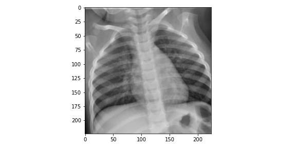
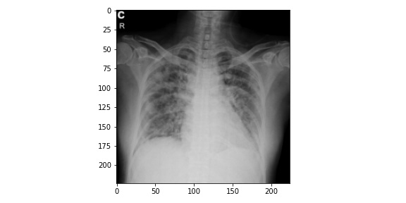
For visualizing an image or set of images, I create a simple helper function. The helper function will visualize both invidiual images and batches of images together.
def viewXRay(img_input, batch=False):

    # Subplots for batches
    if batch:
        fig = plt.figure(figsize=(25,20))
        fig.subplots_adjust(bottom=0.025, left=0.025, top = 0.975, right=0.975)
        plot_dim = len(img_input) // 4
        for i in range(len(img_input)):
            fig.add_subplot(plot_dim, plot_dim, i+1)
            plt.imshow(img_input[i].permute(1, 2, 0))
            plt.tight_layout()

    else:
        fig = plt.figure(figsize=(8,4))
        plt.imshow(img_input.permute(1, 2, 0))
        plt.tight_layout()

    plt.show()
viewXRay(train_dataset[-1][0])
viewXRay(train_dataset[5][0])
1.3. Visualization for Batches
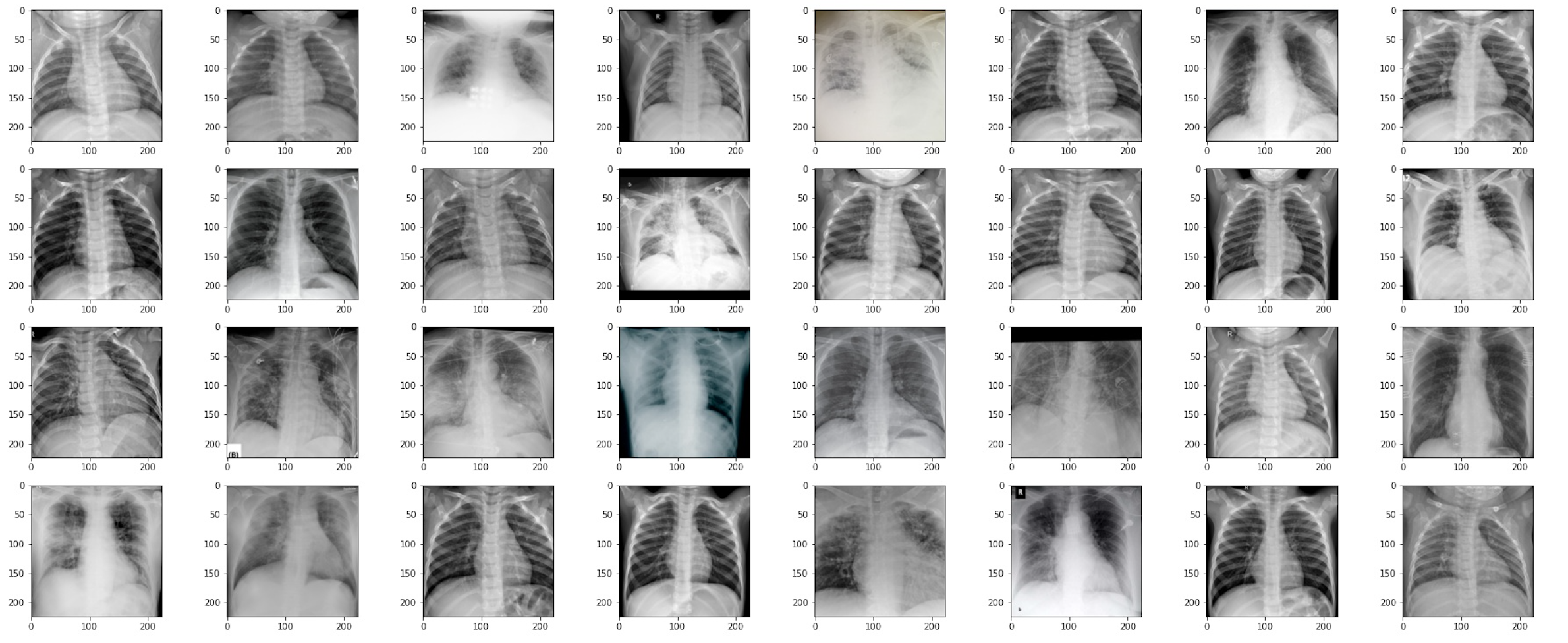
The helper function also covers batch views. This way, we can pass the batch from the dataloader directly into the function and it will return subplots with xray images.
train_dataloader = DataLoader(train_dataset, batch_size=32, shuffle=True)

images, labels = next(iter(train_dataloader))
viewXRay(images, batch=True)
2. Building CNN Model
To the trained eye, these x-ray images may make sense. For the rest of us, leveraging deep learning to learn features in the image may be the best bet in identifying covid x-rays and normal x-rays. The model Architecture I am using will have 3 Convolution Layers and 2 linear layers. I add MaxPooling in the subsequent convolution layer and some dropout layers for regularization.
The implementations of the architecture is available below:
import numpy as np
import torch.nn as nn
import torch.optim as optim

class CovidXRayDetection(nn.Module):

    def __init__(self, n_classes=2):
        super(CovidXRayDetection, self).__init__()
        self.features = nn.Sequential(
            nn.Conv2d( in_channels=3, out_channels=32, kernel_size=3, stride=1),
            nn.ReLU(inplace=True),
            nn.Conv2d( in_channels=32, out_channels=64, kernel_size=3),
            nn.ReLU(inplace=True),
            nn.MaxPool2d(kernel_size=2),
            nn.Dropout(.25),
            nn.Conv2d(in_channels=64, out_channels=128, kernel_size=3),
            nn.ReLU(inplace=True),
            nn.MaxPool2d(kernel_size=2),
            nn.Dropout(.25),
        )

        self.avg_pool = nn.AdaptiveAvgPool2d(2)
        self.classifier = nn.Sequential(
            nn.Linear(128 * 2 * 2, 64),
            nn.ReLU(inplace=True),
            nn.Dropout(.5),
            nn.Linear(64, 1),
        )


    def forward(self, x):
        x = self.features(x)
        x = self.avg_pool(x)
        x = torch.flatten(x, 1)
        x = self.classifier(x)
        return x
3. Model Initialization and Training
To train the model, I have opted to use the Adam optimizer with a learning rate of .01, and the loss function will be Binary Cross Entropy. This is because the target outcomes of the predictions are binary, and using BCEWithLogitsLoss ensures that our model does not produce probabilities. Instead, the probabilities will be calculated using the loss function.
Implementation of the training routine:
# initialize the model
model = CovidXRayDetection()

# parameters
learning_rate = .01
optimizer = optim.Adam( model.parameters(), lr=learning_rate)

# Loss function
loss_function = nn.BCEWithLogitsLoss(reduction='mean', pos_weight=torch.tensor([1.]))

# epochs
epochs = 50
losses = []

for epoch in range(epochs):

    mini_batch_losses =[]
    for x_batch, y_batch in train_dataloader:

        model.train()

        y_pred = model(x_batch)

        loss = loss_function(y_pred, y_batch.unsqueeze(1).float())
        loss.backward()

        optimizer.step()
        optimizer.zero_grad()

        mini_batch_losses.append(loss.item())


    loss = np.mean(mini_batch_losses)
    losses.append(loss)

print(f"Epoch: {epoch}, Loss: {loss}")Epoch: 0, Loss: 0.7217250019311905 Epoch: 1, Loss: 0.7006456106901169 Epoch: 2, Loss: 0.6594521775841713 Epoch: 3, Loss: 0.622551117092371 Epoch: 4, Loss: 0.4777718745172024 Epoch: 5, Loss: 0.42663420736789703 Epoch: 6, Loss: 0.3091115616261959 Epoch: 7, Loss: 0.2671959847211838 Epoch: 8, Loss: 0.26181135699152946 Epoch: 9, Loss: 0.2637191619724035 Epoch: 10, Loss: 0.2649126425385475 Epoch: 11, Loss: 0.2811101209372282 Epoch: 12, Loss: 0.23474631272256374 Epoch: 13, Loss: 0.23240581166464835 Epoch: 14, Loss: 0.24001342244446278 Epoch: 15, Loss: 0.22849101945757866 Epoch: 16, Loss: 0.21720479056239128 Epoch: 17, Loss: 0.19048296194523573 Epoch: 18, Loss: 0.1754478020593524 Epoch: 19, Loss: 0.18594214040786028 Epoch: 20, Loss: 0.20017251884564757 Epoch: 21, Loss: 0.23603381495922804 Epoch: 22, Loss: 0.1866110609844327 Epoch: 23, Loss: 0.20468028541654348 Epoch: 24, Loss: 0.2053750939667225 Epoch: 25, Loss: 0.2322987513616681 Epoch: 26, Loss: 0.1793487872928381 Epoch: 27, Loss: 0.15538806840777397 Epoch: 28, Loss: 0.20436909375712276 Epoch: 29, Loss: 0.19200498051941395 Epoch: 30, Loss: 0.15856635384261608 Epoch: 31, Loss: 0.15390582103282213 Epoch: 32, Loss: 0.19708898663520813 Epoch: 33, Loss: 0.21701610274612904 Epoch: 34, Loss: 0.3220353554934263 Epoch: 35, Loss: 0.24722643941640854 Epoch: 36, Loss: 0.22207679599523544 Epoch: 37, Loss: 0.17871477361768484 Epoch: 38, Loss: 0.15754215978085995 Epoch: 39, Loss: 0.1523445942439139 Epoch: 40, Loss: 0.20394558552652597 Epoch: 41, Loss: 0.2540366337634623 Epoch: 42, Loss: 0.20610464923083782 Epoch: 43, Loss: 0.2029423825442791 Epoch: 44, Loss: 0.2104199305176735 Epoch: 45, Loss: 0.16047851648181677 Epoch: 46, Loss: 0.16203059442341328 Epoch: 47, Loss: 0.1629633717238903 Epoch: 48, Loss: 0.1281860782764852 Epoch: 49, Loss: 0.10838314751163125
fig = plt.figure(figsize=(10,3))

plt.plot(range(1,51) , losses)
plt.title('Model Training Loss by Epoch')
plt.xlabel('Epochs')
plt.ylabel('Loss')
4. Model Prediction
To keep things simple, I have decided not to run the model against a validation set for loss analysis. Instead, I will use the validation set as a test set to evaluate the accuracy of the model. I will assess the model's performance by setting a threshold of .5 for Covid predictions.
validation_dataset = datasets.ImageFolder('data/Val/', transform=transform)
validation_dataloader = DataLoader(validation_dataset, batch_size=32, shuffle=True)
test_predictions, test_outcomes = [], []
model.eval()
for x_input, y_outcomes in validation_dataloader:
# predictions
for pred in (torch.sigmoid(model(x_input)) > .5).squeeze():
test_predictions.append(pred.item())
# outcomes
for outcome in y_outcomes:
test_outcomes.append(outcome.item())import seaborn as sns
from sklearn.metrics import confusion_matrix, roc_curve, precision_recall_curve, auc, accuracy_scoreprint('Accuracy Score:', accuracy_score( test_outcomes, test_predictions, normalize=True)) Accuracy Score: 0.9666666666666667
sns.heatmap(confusion_matrix(test_outcomes, test_predictions), annot=True,)
        plt.title('Test Data Confusion Matrix')
        plt.xlabel('Predicted Labels')
        plt.ylabel('True Labels')
        plt.show()