Data Augmentation for Computer Vision Modeling using torchvision
When building computer vision models, a common task in the data processing pipeline involves performing data transformation and augmentation using transforms. These tasks help normalize the datasets in order to avoid problems with exploding gradients. Additionally, they introduce complexity into the dataset, such as flipping or cropping, to reduce overfitting and lead to more robust models.
In this note, I will discuss the implementation of the following transforms/data augmentation techniques:
- 1. Resizing: This involves standardizing images into similar height and width dimensions.
- 2. Flipping: It changes the image to introduce complexity through rotation, making the model robust.
- 3. Cropping: Random cropping often introduces extra complexity to the images, allowing the model to learn from different parts of the image.
- 4. ColorJitters: Randomized changes to the brightness, contrast, hue, and saturation elements of an image.
- 5. Affline Transforms: Implements a combination of scaling, rotation, translation, and/or shearing to the image.
- 6. Compose: Combining a sequence of transformations into a single operator.
These are just a few examples of transformations performed as part of building a pipeline for deep learning. While you can build these transforms in Python functions, torchvision offers a number of efficiently implemented transformations that can be used on image datasets. This note demonstrates some of the implementations of transformations using the torchvision library.
To begin, let's import the necessary libraries and read in a sample image.
import numpy as np
from torchvision import transforms
from PIL import Image
import matplotlib.pyplot as plt

%matplotlib inline
%config InlineBackend.figure_format = 'retina'

img = Image.open('images/dog.jpg')
img.size
fig = plt.figure(figsize=(7,4))
plt.imshow(img)
plt.show()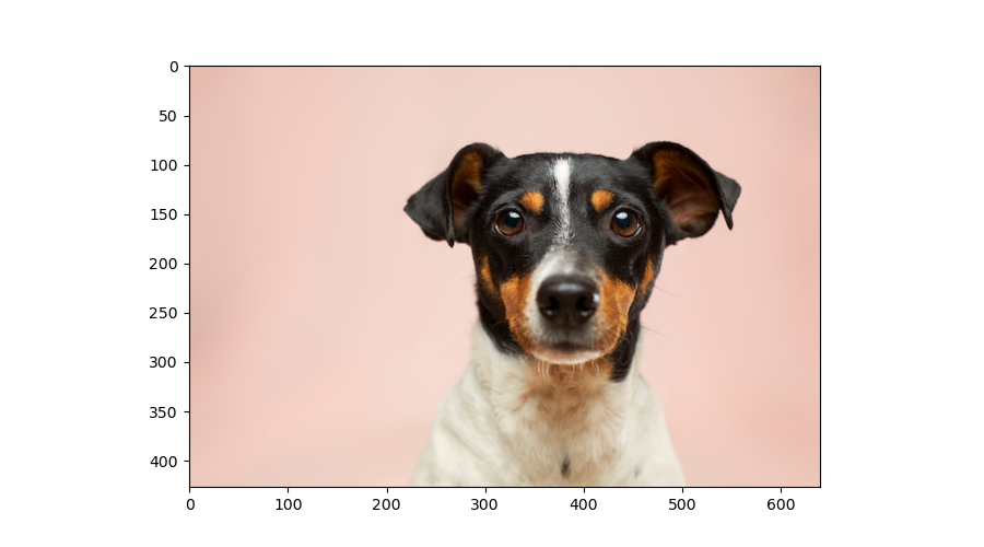
1. Resizing Images
The transform.Resize() method takes an integer or tuple as input and resizes the original image from its initial height $h$ and width $w$ to the target height and width. In this example, I will implement a resize to (150, 200) height and width dimensions.
resize_transform = transforms.Resize( (150, 200))
resized_image = resize_transform(img)

fig = plt.figure(figsize=(7,4))
plt.imshow(resized_image)
plt.show()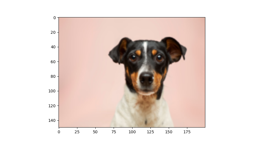
2. Vertical Flip
One approach to augmenting image datasets is to use vertical or horizontal flips. The idea is to train the model to recognize that a dog is still a dog whether it is flipped or not. Torch offers a RandomVerticalFlip() method that takes a probability $p$ for the reflection to occur. The default probability of 50% often works well.
vertical_flip = transforms.RandomVerticalFlip(p=.8)
flipped_imaged = vertical_flip(img)

plt.imshow(flipped_imaged)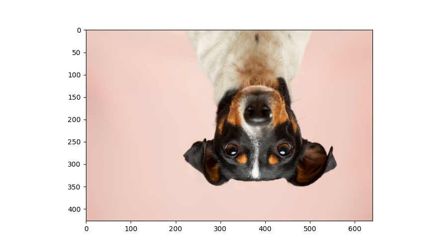
3. Random Crop
Another effective data augmentation technique is to perform random cropping on images. This technique generates a random crop based on the dimensions provided as arguments to the RandomCrop() method. In the example below, we generate random cropped images with dimensions (200, 200).
random_crop = transforms.RandomCrop( (200, 200))
cropped_img = random_crop(img)
plt.imshow(cropped_img)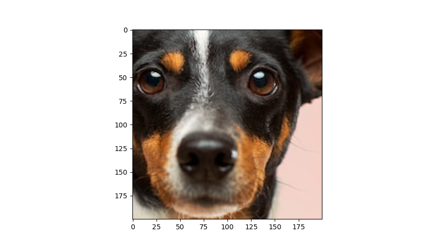
4. ColorJitters
The ColorJitter method implements randomized changes in brightness, contrast, saturation, and hue of an image based on input parameters provided for each of these components. Each parameter takes a value between $0$ and $1$.
colorjitter_transform = transforms.ColorJitter(brightness=.5, contrast=.5, saturation=.5, hue=.5)
color_tranformed_img = colorjitter_transform(img)

plt.imshow(color_tranformed_img)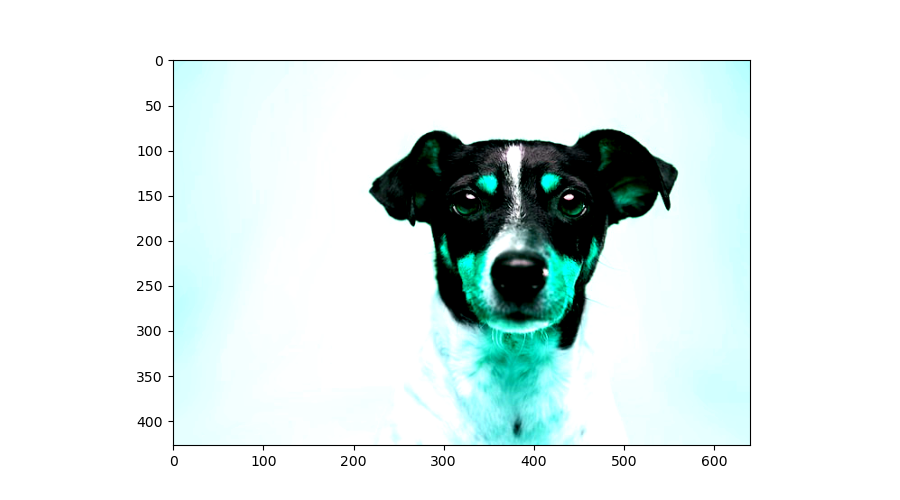
5. Affine Transformation
An Affine Transformation involves four-dimensional changes to an image, including scaling, rotation, translation, and shearing. This transformation can have the effect of changing the plane on which the image was captured. The example below uses a simple transformation with only rotation and shear at 89 degrees and 50, respectively.
affine_transform = transforms.RandomAffine(degrees=89, translate=None, scale=None, shear=50)
affine_img = affine_transform(img)

plt.imshow(affine_img)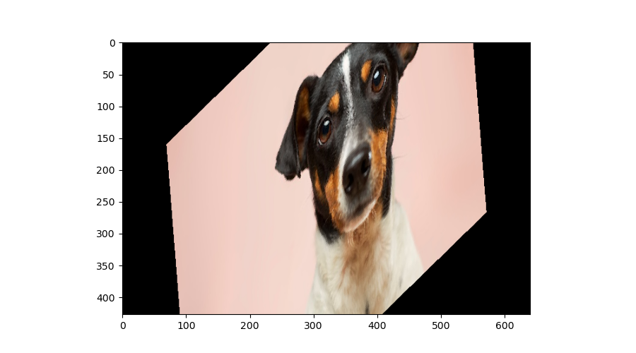
6. Transform Compose
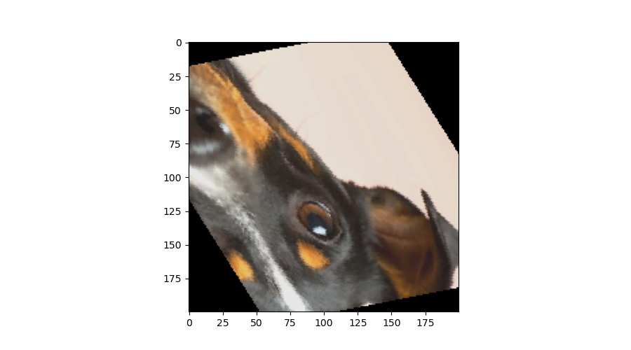
In the above examples, we have seen the power of individual transforms. However, it is common to implement a sequence of transforms on an image. The transform.Compose method allows us to achieve this. The example below implements the sequence of transforms we have seen above.
compose_transform = transforms.Compose( [ transforms.Resize( (450, 500)),
        transforms.RandomVerticalFlip(p=.8),
        transforms.RandomCrop( (200, 200)),
        transforms.ColorJitter(brightness=.5, contrast=.5, saturation=.5, hue=.5) ,
        transforms.RandomAffine(degrees=89, translate=None, scale=None, shear=50) ] )

composed_img = compose_transform(img)
plt.imshow(composed_img)