Classification with Logistic Regression using PyTorch
Logistic Regression is a natural extension of Linear Regression for modeling problems involving categories and classes. In classification, we typically have a finite set of classes or labels associated with data points. For example, while house prices can be virtually unlimited, the sentiment of restaurant reviewers can only have positive, neutral, and negative.
There are several classification techniques suited for varying types of classification problems. On this note, I look at the logistic regression linear classifier and its implementation in PyTorch.
Logistic Regression Model
To intuitively understand the logistic regression model, I begin with the linear model with two variables. Recall, the line model is of the form:
$$ y = \alpha + \beta_1*x_1 + \beta_2*x_2 $$
With the linear model above, there are virtually unlimited possibilities of the outcome variable $y$ for any $x_{1i}$ and $x_{2i}$. The $y$ values can range from $\infty$ to $-\infty$. This of course complicates things because what we need is to be able to tell, given the value of $y$, what class a set of observations belongs to.
We need to find a way to convert the outcome $y$ into distinct classes. This technique of converting infinite values to a finite domain is referred to broadly as generalized functions/models. In the case of classification, we need a function, say $g(y)$ that will convert inputs within the bounds of $0$ and $1$. These are also referred to as probabilities.
Mathematically, this representation is:
$$ g( y ) = g( \alpha + \beta_1*x_1 + \beta_2*x_2 ) = P[y=1| (x_i, x_2)] $$
Sigmoid Function
As it turns out, the sigmoid function does this very well. The sigmoid function takes the form:
$$ sigmoid = \frac {1} {1 + e^{-y}} $$
where:
$y$ is the linear model form.
To demonstrate the usefulness of the sigmoid function, let's plug in the extreme ends of the y possibilities $(-\infty, \infty)$ to it and see the results.
Case 1: $\infty$
$$ sigmoid(\infty) = \frac {1} {1 + e^{-\infty}} = \frac {1} {1 + \frac {1}{e^{\infty}}}$$
$Note: e^{\infty} = \infty$ and $\frac {1}{\infty}$ approximates to $0$, therefore:
$$ sigmoid(\infty) = \frac {1} {1 + \frac {1}{\infty}} = \frac {1} {1 + 0} = \frac {1} {1} = 1 $$
Case 2: $-\infty$
$$ sigmoid(-\infty) = \frac {1} {1 + e^{-{-\infty}}} = \frac {1} {1 + {e^ {\infty}}}$$
$Note: e^{\infty} = \infty$, therefore:
$$ sigmoid(-\infty) = \frac {1} {1 + \infty} = \frac {1} {\infty} = 0 $$
As detailed above, the $sigmoid$ function will generalize extremes to probabilities between $0$ and $1$. We can then set boundaries for classification.
Logistic Regression Model
The logistic regression model for the dataset with two features can be represented by the form:
$$ P[y=1| (x_1, x_2)] = \frac { 1 } { 1 + e^{- y } }$$
Expanding the $y$ input, we get:
$$ P[y=1| (x_1, x_2)] = \frac {1} { 1 + e^{-(\alpha + \beta_1*x_1 + \beta_2*x_2)}} $$
The model returns the probability of the observation being positive $(i.e. 1)$ given features $x_1, x_2$.
With the theory out of the way, let's get to implementing a Logistic Regression model in PyTorch
Generating Classification Data.
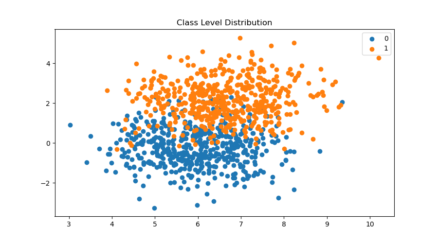
Let's generate some classification data. This can be achieved with the sklearn.datasets make_blobs method.
import numpy as np
import matplotlib.pyplot as plt
from sklearn.datasets import make_blobs

%matplotlib inline
%config InlineBackend.figure_format = 'retina'
To generate classification data, we define the number of classes, number of features, total samples, and random state.
samples = 1000
classes = 2
features = 2

data, labels = make_blobs(n_samples=samples, n_features=features, centers=classes, random_state=261 )
fig = plt.figure(figsize=(12,7))
for label in range(classes):
plt.scatter(data[labels == label, 0], data[labels == label, 1], label=label)
plt.title('Class Level Distribution')
plt.legend()
PyTorch Logistic Regression Model Class
With the data above ready, we can set up a logistic regression model object in PyTorch using nn.Module
import torch
import torch.nn as nn
import torch.optim as optim


class LogisticRegression(nn.Module):

    def __init__(self, features):
        super().__init__()
        self.model = nn.Sequential()
        self.model.add_module('linear', nn.Linear(features, 1))
        self.model.add_module('sigmoid', nn.Sigmoid())

    def forward(self, x):
        return self.model(x)
Initializing Model and Parameters
Next, I initialize the logistic regression model into a linear classifier object.
torch.manual_seed(420)

linear_classifier = LogisticRegression(2)
linear_classifier.state_dict()OrderedDict([('model.linear.weight', tensor([[ 0.4318, -0.4256]])),
('model.linear.bias', tensor([0.6730]))])I can now set up the learning parameters and optimizer.
learning_rate = .1
optimizer = optim.SGD(linear_classifier.parameters(), lr=learning_rate)
Loss Function: Binary Cross Entropy
The Binary Cross Entropy function takes the form:
$$ BCE = \frac {-1}{ N_{pos} + N_{neg}} \left[ \sum_{i=1}^N log(P(y_i = 1)) + \sum_{i=1}^N log(1 - P(y_i = 1)) \right] $$
At first glance the formula can be rather unintuitive, however with a little exploration of logarithms and probabilities, we discover that BCE is the average of negative log losses. Let's see BCE more intuitively.
We know that the logistic regression will return probabilities as outcomes with high probability values as positive prediction and vice versa. We also know that probabilities range from $0$ to $1$. It turns out that logarithm has a nice property that works well with probabilities.
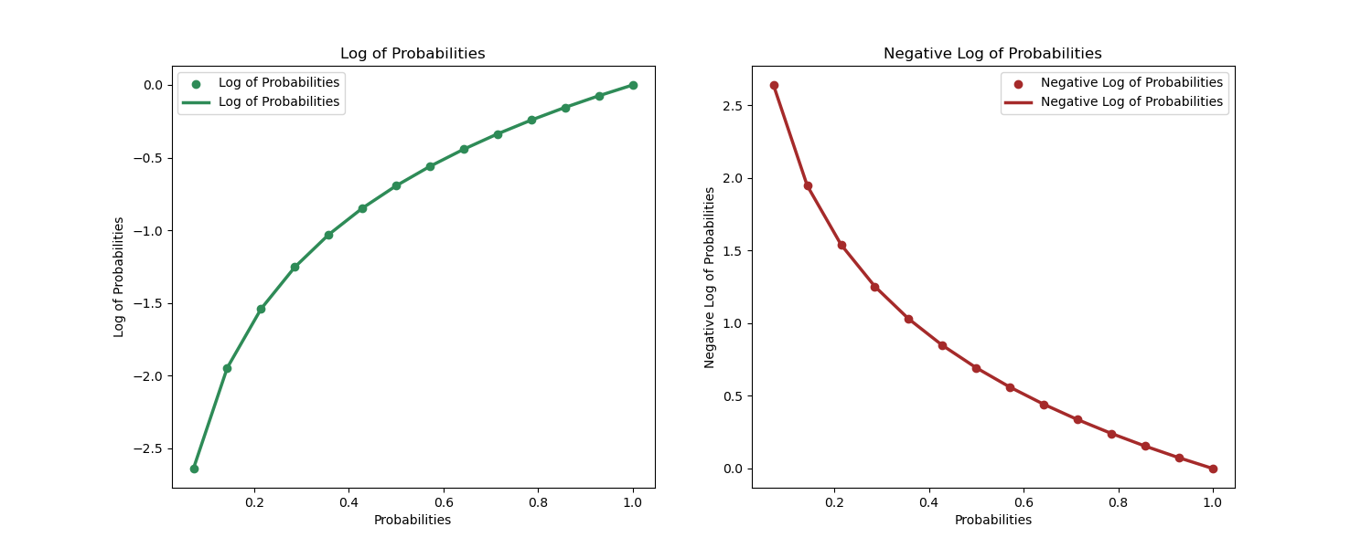
When the probability of an observation is closer to 1, $P(y_i = 1| (x_i))= 1$, then the log of the probability is $log(P(y_i = 1| (x_i)))= log(1) = 0$
When the probability of an observation is closer to 0, $P(y_i = 1| (x_i))= .2$, then the log of the probability is $log(P(y_i = 1| (x_i)))= log(.2) = -1.6$
This property of logarithms to probabilities has two neat implications that make it very useful as a loss function.
- 1. When our model has correctly predicted the positive class, $P(y_i = 1| (x_i))= 1$, then the loss is exactly $0$. This is exactly what we want our loss function to do.
- 2. Using the negative log, we can convert the loss values and use them to train weights much like the case for linear regression.
Below is a simple demonstration of the log and negative log against probabilities.
import numpy as np
import matplotlib.pyplot as plt

# probabilities
x = np.linspace(0, 1, 15)

# log and negative log visualization
fig = plt.figure(figsize=(20,8))

plt.subplot(121)
plt.scatter(x, np.log(x), label='Log of Probabilities', color='seagreen')
plt.plot(x, np.log(x), label='Log of Probabilities', color='seagreen', linewidth=2.5)
plt.title('Log of Probabilities')
plt.xlabel('Probabilities')
plt.ylabel('Log of Probabilities')
plt.legend()

plt.subplot(122)
plt.scatter(x, -1*np.log(x), label='Negative Log of Probabilities', color='brown')
plt.plot(x, -1*np.log(x), label='Negative Log of Probabilities', color='brown', linewidth=2.5)
plt.title('Negative Log of Probabilities')
plt.xlabel('Probabilities')
plt.ylabel('Negative Log of Probabilities')
plt.legend()

plt.show()
From the demonstration above, we can begin to understand intuitively why this loss function works for binary classification problems.
BCE with PyTorch
There are two implementations of BCE in Pytorch.
- 1. nn.BCELoss: This function expects probabilities to be passed on. This means that your model architecture must have a Sigmoid activation function.
- 2. nn.BCEWithLogitLoss: Thie function expects non-probability predictions and computes their probabilities and loss within the function. If you are using this function, you should not have Sigmoid layers on your model architecture.
loss_function_1  = nn.BCELoss(reduction='mean')
loss_function_2 = nn.BCEWithLogitsLoss(reduction='mean', pos_weight=torch.tensor([1.]))
Putting Everything Together
We now have all the elements we need to train a linear classifier. Below is the implementation including Dataset, Model and Training Loop.
import torch
import torch.nn as nn
import torch.optim as optim

import numpy as np
from sklearn.datasets import make_blobs

from torch.utils.data import Dataset, DataLoader, random_split
1. Dataset, Train-Test Split, and Data Loader Setup
1.1. Dataset Class
PyTorch uses the dataset and data loader class for iterative batch training and backpropagation. Here we define the dataset, train test split, and data loader setup.
# Creating the Dataset and Model Classes

class BinaryClassData(Dataset):

    def __init__(self, x_input, y_output):
        self.x_input = x_input
        self.y_output = y_output

    def __getitem__(self, index):
        if index >= len(self.x_input):
            return "Value does not exist"
        return (self.x_input[index], self.y_output[index])

    def __len__(self):
        return len(self.x_input)
samples = 1000
classes = 2
features = 2
# generating data and converting to tensors
x_inputs, y_output = make_blobs(n_samples=samples, n_features=features, centers=classes, random_state=261 )
x_inputs, y_output = torch.from_numpy(x_inputs), torch.from_numpy(y_output)
x_inputs, y_output = x_inputs.type(torch.FloatTensor), y_output.type(torch.FloatTensor)
# Initialize the data
binary_data = BinaryClassData(x_inputs, y_output)len(binary_data), binary_data[5](1000, (tensor([8.4116, 3.8735]), tensor(1.)))
1.2. Train Test Split
train_set, test_set = random_split(binary_data, [800, 200])
len(train_set), train_set[5], len(test_set), test_set[5](800, (tensor([ 5.4493, -1.9747]), tensor(0.)), 200, (tensor([ 5.6047, -1.2734]), tensor(0.)))
1.3. DataLoader Setup
train_data_loader = DataLoader(dataset=train_set, batch_size=16, shuffle=True)
test_data_loader = DataLoader(dataset=test_set, batch_size=16, shuffle=True)
2. Model Configuration
For the logistic regression model, we will use a linear architecture with a BCEWithLogitLoss function for probability estimations. This means that we will still evaluate the loss with the Sigmoid function but it won't be defined in the model class.
class LogisticRegression(nn.Module):

    def __init__(self, input_features):
        super(LogisticRegression, self).__init__()
        self.model = nn.Linear(input_features, 1)

    def forward(self, x):
            return self.model(x)
torch.manual_seed(420)
# initialize model
model = LogisticRegression(2)
model.state_dict()OrderedDict([('model.weight', tensor([[ 0.4318, -0.4256]])),
('model.bias', tensor([0.6730]))])3. Training Loop
We have everything we need to complete our training loop.
learning_rate = .1
optimizer = optim.SGD(model.parameters(), lr=learning_rate)

bce_with_logit_loss = nn.BCEWithLogitsLoss(reduction='mean', pos_weight=torch.tensor([1.]))

epochs = 100
losses = []

for epoch in range(epochs):

    mini_batch_losses = []
    for x_batch, y_batch in train_data_loader:

        model.train()

        y_pred = model(x_batch)

        loss = bce_with_logit_loss(y_pred, y_batch.unsqueeze(1))
        loss.backward()

        optimizer.step()
        optimizer.zero_grad()

        mini_batch_losses.append(loss.item())

    loss = np.mean(mini_batch_losses)
    losses.append(loss)


model.state_dict()OrderedDict([('model.weight', tensor([[0.2822, 2.5435]])),
('model.bias', tensor([-3.7672]))])4. Model Training Loss
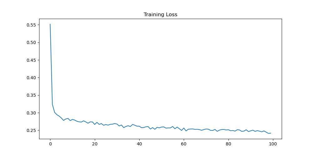
With the model training completed, we can visualize the loss training logged in the loss array.
fig = plt.figure(figsize=(10, 5))
plt.plot(losses)
plt.title('Training Loss')
5. Test Predictions and Confusion Matrix
We can now run predictions and model evaluation on the test data. Recall that our model returns logits and we therefore have to apply the sigmoid activation function to convert logits to probabilities. In the example below, we set the classification threshold at $.5$.
model.eval()LogisticRegression( (model): Linear(in_features=2, out_features=1, bias=True) )
test_predictions, test_outcomes = [], []

for x_input, y_outcomes in test_data_loader:

    # predictions
    for pred in (torch.sigmoid(model(x_input)) > .5).squeeze():
        test_predictions.append(pred.item())

    # outcomes
    for outcome in y_outcomes:
            test_outcomes.append(outcome.item())
5.1 Confusion Matrix
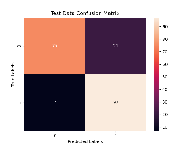
The confusion matrix helps us understand the quality of our predictions. That is how many correct and wrong predictions we made given our model parameters. Below, we visualize the confusion matrix.
import seaborn as sns
from sklearn.metrics import confusion_matrix, roc_curve, precision_recall_curve, auc, accuracy_score


print('Confusion Matrix:', confusion_matrix(test_outcomes, test_predictions))
print('Accuracy Score:', accuracy_score( test_outcomes, test_predictions, normalize=True))Confusion Matrix: [[75 21]
[ 7 97]]
Accuracy Score: 0.86sns.heatmap(confusion_matrix(test_outcomes, test_predictions), annot=True,)
plt.title('Test Data Confusion Matrix')
plt.xlabel('Predicted Labels')
plt.ylabel('True Labels')
plt.show()
For a linear classifier, our accuracy score at $86%$ is very good. With a little improvement such as adding layers which effectively add dimensions to draw the hypherplane for classification, we can improve the accuracy.
Beyond Accuracy: Quality of the Model
In classification, there are several useful metrics that provide details about the model performace beyond accuracy. These metrics are:
1. False Positive Rate:
This is percent misclassification of positive outcomes for all negative observations. That is, of the known negative observation, how many observertions did the model classify as positive.
$$ FPR = \frac {FP} {FP + TN} $$
2. Precision
Precision measurement tells us of the positive predictions from the model, how many of those predictions were correct. Mathametically, it is represented as:
$$ precision = \frac {TP} {TP + FP} $$
3. Recall
Recall is much like the True positive rate. It tells us of all the positive observations, how many of the did we predict correctly. Mathematically, it is expressed as:
$$ recall = \frac {TP} {TP + FN} $$
The implementation of these metrics in python is given below:
def classification_metrics(confusion_matrix):

    # negatives and positives
    negatives, positives = confusion_matrix[0], confusion_matrix[1]
    true_negative, false_negative = negatives[0], positives[1]
    true_positive, false_positive = positives[0], negatives[1]

    # metrics
    fpr = false_positive/(false_positive + true_negative)
    precision = true_positive/(true_positive + false_positive)
    recall = true_positive/(true_positive + false_negative)

    return fpr, precision, recall
classification_metrics( confusion_matrix(test_outcomes, test_predictions) )(0.21875, 0.25, 0.0673076923076923)