Classification with k-Nearest Neighbor
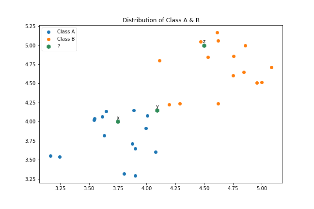
Suppose we have a dataset consisting of x and y variables representing two known classes, A and B, where class A is denoted by blue points and class B by orange points.

Classifying points $x$ and $y$ to class $A$ and $B$, respectively, with a high degree of certainty is perhaps more straightforward. However, when it comes to point $y$, one may have to take a chance and assign it to either class. In all three cases, the assumption is that the nearest known points to the unknown point provide valuable information to determine the class of the unknown point. This is the fundamental idea behind k-Nearest Neighbors.
For point $y$, if there is an almost equal number of nearest known points from class $A$ and $B$, it can reduce our confidence in the classification, but the rationale behind this approach remains valid.
K-Nearest Neighbors
K-Nearest Neighbors is one of the more intuitive learning techniques in Machine Learning. In many ways, the approach mirrors how we generally estimate or assess the value of products or services in that we often look at comparable items to determine the value of a product or service. Suppose that you are a homeowner who is selling your house or better yet you are interested in purchasing a house, how do you assess the value of the house?
A common practice would be to find a set of houses that are the most similar to the house of interest and use that information to assign value. Some of these similarity features may be location, square footage, number of bedrooms, and proximity to business centers and schools among others. In fact, it is often the case that in real-world neighborhoods, housing prices are often comparable on similar properties. This is the intuition behind K-Nearest Neighbors.
What is KNN?
K-Nearest Neighbors is a non-parametric technique that returns a prediction of an input based on the $k$ most similar observations. It is non-parametric because it does not compute parameters as is the case of linear regression. This gives the technique some useful advantages such as not requiring to make assumptions about the distribution of the data. Its simplicity makes it easy to understand and implement, and it performs incredibly well for complex relationships,s, particularly as $k$ increases. KNN can also be used for classification and regression problems with little modification.
At the core of the KNN technique is the idea that observations with similar features are likely to have similar target variables. Therefore, to make a prediction of a query input we only need find the most similar observations to predict the input's class or target variable. So how do we determine what observations are similar to the input?
Distance Metrics
There are various classes of distance metrics that can be used to determine the similarity between observations. On this note, we focus on two of the most common geometric distances: Euclidean Distance and Cosine Similarity
1. Euclidean Distance
The Euclidean distance is the most commonly used geometric distance metric. It returns the distance between points in a vector space. Mathematically, the Euclidean distance is given as:
$$ d(x, y) = \sqrt { \sum_{i=1}^n (x_i - y_i)^2 } $$
where $x$ and $y$ are vectors.
The expanded form of the equation is for two points in a 2-D vector space is:
$$ d(x, y) = \sqrt { (x_1 - x_2)^2 + (y_1 - y_2)^2 } $$
For example, suppose we have two points:
A = (6.3, 4.1)
B = (3.2, 1.7)
The Euclidean distance between the two points is given by:
$$ d(A,B) = \sqrt { (6.3 - 3.2)^2 + (4.1 - 1.7)^2 } $$ $$ d(A,B) = \sqrt { (3.1)^2 + (2.4)^2 }$$ $$ d(A, B) = \sqrt { (9.6) + (5.76) } = \sqrt { 15.369 } = 3.92 $$
Implementation with python code:
import numpy as np

a = np.array([6.3, 4.1])
b = np.array([3.2, 1.7])

d = np.sqrt( np.sum( (a - b)**2 ) )
d3.920459156782531
Cosine Similarity
The cosine similarity is the measure of similarity between two vectors. More precisely, it is the cosine measure of the angle between two vectors.
Mathematically, it is represented as:
$$ d(a,b) = \frac{ a*b } { |a| |b| } $$
where:
$a*b$ is the dot product of vectors
$ |a|$ and $|b|$ are the dot products of the vectors
The formula can be expanded on with summation definitions as follows:
$$ d(a, b) = \frac { \sum_{i=1}^n {a_i b_i} } { \sqrt { \sum_{i=1}^n {a_i^2}} \sqrt {\sum_{i=1}^n{b_i^2}} } $$
For example:
$$ d(a, b) = \frac { (6.3*3.2) + (4.1*1.7) } { \sqrt { (6.3^2) + (4.1^2)} \sqrt { (3.2^2) + (1.7^2) } } $$ $$ d(a, b) = \frac {27.13} { 7.516 * 3.623} $$ $$ d(a, b) = \frac {27.13} {27.2368} $$ $$ d(a, b) = .996 $$
np.dot(a, b)/(np.sqrt(np.dot(a, a)) * np.sqrt( np.dot(b, b) ))0.9960776759242224
Choosing Optimal $k$
After understanding Nearest Neighbors and distance computation, the crucial question is determining the optimal value for $k$, i.e., the number of neighbors to consider for predicting the class of a new observation. Common heuristics include selecting an odd or odd prime number, ensuring that the predicted outcome is always a single class. Additionally, other rules involve using the number of classes in the dataset and adding one if the total number of classes is even. In this example, we will use the prediction error rate to suggest the appropriate class.
kNN Algorithm
Let's implement the KNN algorithm. Using pseudo-code, the kNN algorithm follows the following implementation details. Note that my implementation leverages objects and the steps may look different if you are building the algorithm functionally.
- 1. Initialize the features and labels of the known observations and k_nearest neighbors
- 2. Initialize input of unknown input vector, size of known observations, and a dict variable to store nearest k neighbors
- 3. Define the Euclidean distance method
Here is where the algorithm really begins:
- 1. Iterate through individual known observations and compute the distance between that observation and unknown input
- 2. Save the distance into a distance variable
- 3. Check if the size of the nearest neighbor dictionary in #2 is equal to or greater than k_nearest_neighbors. If the size is not equal or greater, add the new distance and neighbor
- 4. If true, sort the nearest neighbor dictionary by value in ascending order
- 5. Check if the distance calculated is lower than the largest distance. If higher, drop the last item in the dictionary and append the new distance. If not pass.
- 6. Return the nearest neighbor dictionary
Implementation in Python
In Python, the implementation looks like below:
import numpy as np

class kNN:

    def __init__(self, features, labels, input_x, k_neighbors=3):
        # Known inputs features and classes
        self.features = features
        self.labels = labels
        self.n_obs = features.shape[1]

        # input to predict
        self.input_x = input_x

        # nearest neighbor
        self.k_neighbors = k_neighbors
        self.nearest_neighbors = {}

    def euclidean_distance(self, arr_1 , arr_2 ):
        return np.sqrt( np.sum( ( arr_1 - arr_2 )**2  ) )


    def k_nearest_neighbors(self):
        for obs in range(self.n_obs):
            distance = self.euclidean_distance(self.input_x, self.features[:, obs])

            if len(self.nearest_neighbors) >= self.k_neighbors:
                self.nearest_neighbors = {k:v for k,v in sorted(self.nearest_neighbors.items(), key=lambda x:x[1])}
                if distance < list(self.nearest_neighbors.values())[-1]:
                    self.nearest_neighbors.popitem()
                    self.nearest_neighbors[obs] = distance
                else:
                    pass

            # When nearest neighbors are less than k_neighbors parameter
            else:
                self.nearest_neighbors[obs] = distance

        return self.nearest_neighbors


    def predict_class(self):
        self.k_nearest_neighbors()
        predicted_labels = [self.labels[index] for index in self.nearest_neighbors.keys()]
        majority_class = {label : predicted_labels.count(label)  for label in set(predicted_labels)}
        for k,v in majority_class.items():
            if v == max(majority_class.values()):
                return f"Predicted Class: {k} \n Nearest Neighbor Distances: {majority_class}"
Implementing the algorithm on Classification Problem
Let's implement our algorithm on a classification problem that we encountered earlier in the note. Below is the code that imports that data and runs the knn-classifier
import pandas as pd
import numpy as np
import matplotlib.pyplot as plt

%matplotlib inline
%config InlineBackend.figure_format = 'retina'
dataset = pd.read_csv('fiction.csv')
dataset.head()| x | y | class | |
|---|---|---|---|
| 0 | 3.649925 | 4.133025 | A |
| 1 | 3.900977 | 3.292829 | A |
| 2 | 4.077340 | 3.603936 | A |
| 3 | 3.546743 | 4.040555 | A |
| 4 | 3.164847 | 3.552950 | A |
fig = plt.figure(figsize=(9,6))
plt.scatter(dataset[dataset.classes=='A' ]['x'], dataset[dataset.classes == 'A']['y'], label='Class A ')
plt.scatter(dataset[dataset.classes=='B' ]['x'], dataset[dataset.classes == 'B']['y'], label='Class B ')


plt.scatter( np.array([3.75, 4.09, 4.5]), np.array([4.0, 4.15, 5.0]), label='?', marker='h', linewidths=3, color='seagreen')
plt.annotate('x', (3.74, 4.03 ) )
plt.annotate('y', (4.08, 4.18 ) )
plt.annotate('z', (4.49, 5.03 ) )


plt.legend(loc='upper left')
plt.title('Distribution of Class A & B')
Running kNN Classifier
To run the kNN algorithm, we initialize the three unknown data points as $x_inputs$.
x_inputs = np.array([[3.75, 4.0] , [4.09, 4.15], [4.5, 5.0] ])
x_inputsarray([[3.75, 4. ],
[4.09, 4.15],
[4.5 , 5. ]])Below, we loop through the $x$_$inputs$ and run the kNN classifier. Notice that we convert the dataset inputs into a 2-D array as we initialize the kNN class.
for x_input in x_inputs:
    knn_model = kNN(np.array([dataset.x, dataset.y]), dataset['classes'].to_numpy(), x_input, k_neighbors=3)
print(knn_model.predict_class())Predicted Class: A
Nearest Neighbor Distances: {'A': 3}
Predicted Class: A
Nearest Neighbor Distances: {'A': 2, 'B': 1}
Predicted Class: B
Nearest Neighbor Distances: {'B': 3}kNN with ScikitLearn
In the real world, you will likely use kNN classifier with scikitlearn for many reasons. It plays well with numpy, has robust implementations and varied distance metrics, and integrates well with other Python computing functionalities. For this reason, I share an example of kNN with scikitlearn. In the following example, we use a wine dataset that can be found here
We begin by importing data into a pandas variable and performing some basic exploration.
wine_data = pd.read_csv('wine.data', header=None)col_names = ['class', 'alcohol', 'malic_acid', 'ash', 'alcalinity_of_ash', 'magnesium', 'total_phenols', 'flavanoids',
'nonflavanoid_phenols', 'proanthocyanins', 'color_intensity', 'hue', 'diluted_wines', 'proline']
wine_data.columns = col_nameswine_data.head()| class | alcohol | malic_acid | ash | alcalinity_of_ash | magnesium | total_phenols | flavanoids | nonflavanoid_phenols | proanthocyanins | color_intensity | hue | diluted_wines | proline | |
|---|---|---|---|---|---|---|---|---|---|---|---|---|---|---|
| 0 | 1 | 14.23 | 1.71 | 2.43 | 15.6 | 127 | 2.80 | 3.06 | 0.28 | 2.29 | 5.64 | 1.04 | 3.92 | 1065 |
| 1 | 1 | 13.20 | 1.78 | 2.14 | 11.2 | 100 | 2.65 | 2.76 | 0.26 | 1.28 | 4.38 | 1.05 | 3.40 | 1050 |
| 2 | 1 | 13.16 | 2.36 | 2.67 | 18.6 | 101 | 2.80 | 3.24 | 0.30 | 2.81 | 5.68 | 1.03 | 3.17 | 1185 |
| 3 | 1 | 14.37 | 1.95 | 2.50 | 16.8 | 113 | 3.85 | 3.49 | 0.24 | 2.18 | 7.80 | 0.86 | 3.45 | 1480 |
| 4 | 1 | 13.24 | 2.59 | 2.87 | 21.0 | 118 | 2.80 | 2.69 | 0.39 | 1.82 | 4.32 | 1.04 | 2.93 | 735 |
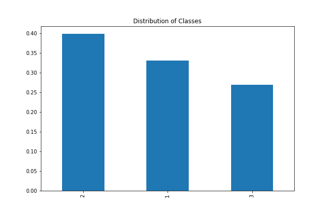
Let's quickly check the distribution of classes in our dataset.
wine_data['class'].value_counts(normalize=True).plot(kind='bar', figsize=(9, 6), title='Distribution of Classes')
plt.savefig('knn-class-distribution.png')
The distribution isn't significantly heavy on one class so we can go ahead and use our kNN class.
Scaling the Dataset with StandardScaler
kNN uses distance metrics. The Euclidean distance metrics are sensitive to the magnitude of vectors, therefore scaling our features will improve its performance. We use the StandardScaler to scale our features below.
from sklearn.preprocessing import StandardScaler

features = wine_data[ [ col for col in col_names if col != 'class' ]]
scaled_features = StandardScaler().fit_transform(features)
Splitting the data into Train and Test
With scaling out of the way, we can now split the data into training and test sets.
Running the kNN Classifier
Our dataset is ready for classification. Below, we run the kNN classifier using $k=3$. We will also compute the accuracy of the test set.
from sklearn.neighbors import KNeighborsClassifier
from sklearn.metrics import accuracy_score

# initializing model
knn_model = KNeighborsClassifier(n_neighbors=3, p=2, metric='minkowski')
knn_model.fit(x_train, y_train)KNeighborsClassifier(n_neighbors=3)
y_pred = knn_model.predict(x_test)
accuracy_score(y_pred, y_test)0.6481481481481481
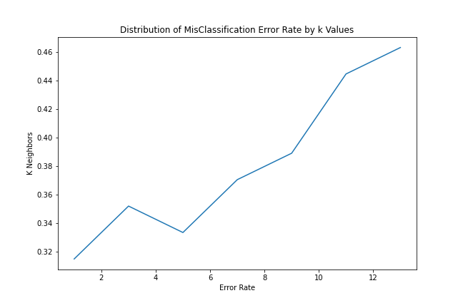
Our test accuracy at $k=3$ is 64%. To see performance at different $k$ values, we run a loop over different $k$ values and assess performance.
k_values = [ k for k in range(15) if k % 2 != 0 ]accuracy = []
for k in k_values:
knn_model = KNeighborsClassifier(n_neighbors=k, p=2, metric='minkowski')
knn_model.fit(x_train, y_train)
y_pred = knn_model.predict(x_test)
accuracy.append(accuracy_score(y_pred, y_test))Plotting the kNN Error Rate
Below, we plot the distribution of $k$ to error rate.
error_rate = [ 1 - x for x in accuracy ]

fig = plt.figure(figsize=(9, 6))
plt.plot(k_values, error_rate)
plt.title('Distribution of MisClassification Error Rate by k Values')
plt.ylabel('K Neighbors')
plt.xlabel('Error Rate')
plt.savefig('knn-error-rate.png')