Binary Cross Entropy Loss Function for Classification
This short note breaks down the Binary Cross Entropy Loss function often used in classification tasks in deep learning.
The Binary Cross Entropy function takes the form:
$$ BCE = \frac {-1}{ N_{pos} + N_{neg}} \left[ \sum_{i=1}^N log(P(y_i = 1)) + \sum_{i=1}^N log(1 - P(y_i = 1)) \right] $$
At first glance the formula can feel rather unintuitive, however with a little exploration of logarithms and probabilities, we discover that BCE is the average of negative log losses. Let's see BCE more intuitively.
For a classification model that predicts a positive and negative outcome, we know that the models will return probability values as outcomes with high probability values as positive prediction and low vice versa. We also know that probabilities range from $0$ to $1$. It turns out that logarithm has a nice property that works well with probabilities.
So What's Happening Here?
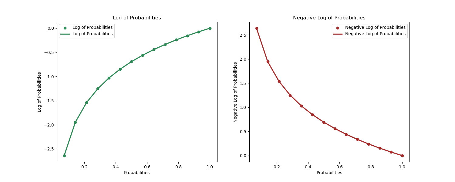
When the probability of an observation is closer to 1, $P(y_i = 1| (x_i))= 1$, then the log of the probability is $log(P(y_i = 1| (x_i)))= log(1) = 0$
When the probability of an observation is closer to 0, $P(y_i = 1| (x_i))= .2$, then the log of the probability is $log(P(y_i = 1| (x_i)))= log(.2) = -1.6$
This property of logarithms to probabilities has two neat implications that make it very useful as a loss function.
- 1. When our model has correctly predicted the positive class, $P(y_i = 1| (x_i))= 1$, the our loss is exactly $0$. This is exactly what we want our loss function to do.
- 2. Using the negative log, we can convert the loss values and use them to train weights much like the case for linear regression.
Below is a simple demonstration of the log and negative log against probabilities.
import numpy as np
import matplotlib.pyplot as plt

# probabilities
x = np.linspace(0, 1, 15)

# log and negative log visualization
fig = plt.figure(figsize=(15,6))

plt.subplot(121)
plt.scatter(x, np.log(x), label='Log of Probabilities', color='seagreen')
plt.plot(x, np.log(x), label='Log of Probabilities', color='seagreen', linewidth=2.5)
plt.title('Log of Probabilities')
plt.xlabel('Probabilities')
plt.ylabel('Log of Probabilities')
plt.legend()

plt.subplot(122)
plt.scatter(x, -1*np.log(x), label='Negative Log of Probabilities', color='brown')
plt.plot(x, -1*np.log(x), label='Negative Log of Probabilities', color='brown', linewidth=2.5)
plt.title('Negative Log of Probabilities')
plt.xlabel('Probabilities')
plt.ylabel('Negative Log of Probabilities')
plt.legend()


plt.show()