Bayesian Time Series Forecasting with PyBats
Bayesian forecasting methods are an effective alternative to traditional frequentist forecasting methods, such as ARIMA methods, as they offer more transparent parameter estimation and robust models. The complexity of estimation can make them less straightforward to understand, but with some understanding of Bayesian logic and experimentation, they turn out to be more intuitive and flexible than frequentist methods.

Bayesian Intuition and Theorem
Bayesian logic begins with the assertion that we have some prior belief about how the world works (e.g., stock prices, air travel, etc.). As we encounter more and more evidence through data observations, we update our beliefs about the nature of the world (posterior beliefs). This can be translated into a formula:
$$ \text{posterior beliefs} = \text{prior belief} * \text{evidence from the data} $$
The Bayes theorem is an approximate translation of this intuition using probabilities. The Bayes theorem is mathematically represented as:
$$ P(A|B) = P(A) * \frac { P(B|A) } { P(B)} $$
where $P(A|B)$ is the posterior distribution (probability of A happening given B has happened), $P(A)$ is the prior distribution, $P(B|A)$ is the likelihood (observation in the data given our prior), and $P(B)$ is the probability of event B (a normalizer for observations to update the prior distribution).
Bayesian Prior and Posterior Distribution
Bayesian methods require priors to be set ahead of any model training, reflecting our initial beliefs about how the data is related. The priors will be updated through training to return posterior distributions. In fact, Bayesian methods don't return point estimates; rather, they return distributions of parameters that can be sampled to generate a forecast and confidence intervals.
A good understanding of some common distributions may be useful. However, most modern forecasting tools, like Prophet and BSTS, have abstracted techniques to take care of this for us. In this simple example, we will use the PyBats tool to develop a Bayesian forecast using a Poisson distribution. For more details on the distribution, see the following note:
Dataset: Time Series Stock Price
For this task, I'll use the stock price dataset to build a bayesian time series forecast. The data is available here:
import numpy as np
import pandas as pd
import matplotlib.pyplot as plt


%matplotlib inline
%config InlineBackend.figure_format = 'retina'
data = pd.read_csv('data.csv')
data = data.tail(-4)
data['date'] = pd.to_datetime(data['date'], format='%Y-%m-%d')
data.head()| date | open_price | high_price | low_price | close_price | volume | adjclose_price | |
|---|---|---|---|---|---|---|---|
| 4 | 2021-01-22 | 42.590000 | 76.760002 | 42.320000 | 65.010002 | 196784300.0 | 65.010002 |
| 5 | 2021-01-21 | 39.230000 | 44.750000 | 37.000000 | 43.029999 | 57079800.0 | 43.029999 |
| 6 | 2021-01-20 | 37.369999 | 41.189999 | 36.060001 | 39.119999 | 33471800.0 | 39.119999 |
| 7 | 2021-01-19 | 41.549999 | 45.520000 | 36.639999 | 39.360001 | 74721900.0 | 39.360001 |
| 8 | 2021-01-15 | 38.490002 | 40.750000 | 34.009998 | 35.500000 | 46752200.0 | 35.500000 |
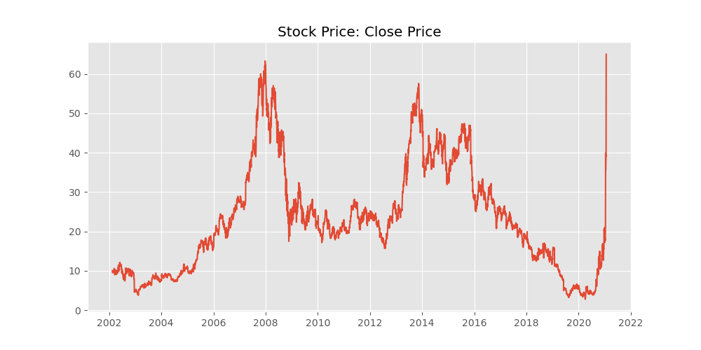
Extracting the close price data for visualization and modeling.
close_data = data[['date', 'close_price']].copy()
close_data.set_index('date', inplace=True)
close_data.head()| close_price | |
|---|---|
| date | |
| 2021-01-22 | 65.010002 |
| 2021-01-21 | 43.029999 |
| 2021-01-20 | 39.119999 |
| 2021-01-19 | 39.360001 |
| 2021-01-15 | 35.500000 |
plt.style.use('ggplot')

fig = plt.figure(figsize=(10, 5))
plt.plot(data.date, data.close_price)
plt.title('Stock Price: Close Price')
plt.show()
Initializing Model with PyBATS
PyBATS is one of the many available packages for Bayesian Structural Time Series models and forecasting. Specifically, PyBATS uses Dynamic Generalized Linear models to model the state spaces of the time series components (trend, seasonality, and autoregressors) as they evolve over time.
Mathematically, DGL model components can be expressed as the multiplicative effect of the state vector by the regression vector:
$$ \lambda{_t} = F{'}{_t} \theta_t $$
where:
- $\lambda{_t}$ is the linear predictor
- $\theta_t$ is the state vector
- $F_t$ is the regression vector.
For further details, see notes on: https://lavinei.github.io/pybats/
The model is initialized with several components, and their significance is commented alongside the input parameters.
from pybats.analysis import analysis
from pybats.point_forecast import mean, median


forecast_step = 1
forecast_start = 0
forecast_end = len(close_data['close_price']) - 1

model, samples = analysis( close_data['close_price'],
                            family='poisson',
                            forecast_start=forecast_start,   # First time step to forecast on
                            forecast_end=forecast_end,       # Final time step to forecast on
                            k=forecast_step,                 # Forecaset Horizon
                            nsamps= 200,                     # Model Outcome Sampling
                            prior_length= 3,                 # Data points used to defining bayesian priors
                            rho = .9,                        # Random effect to increase robustness of model through variance
                            deltrend=.5,                     # Regularized for Intercept Component
                            delregn=.9 )                     # Regularized for Regression Component
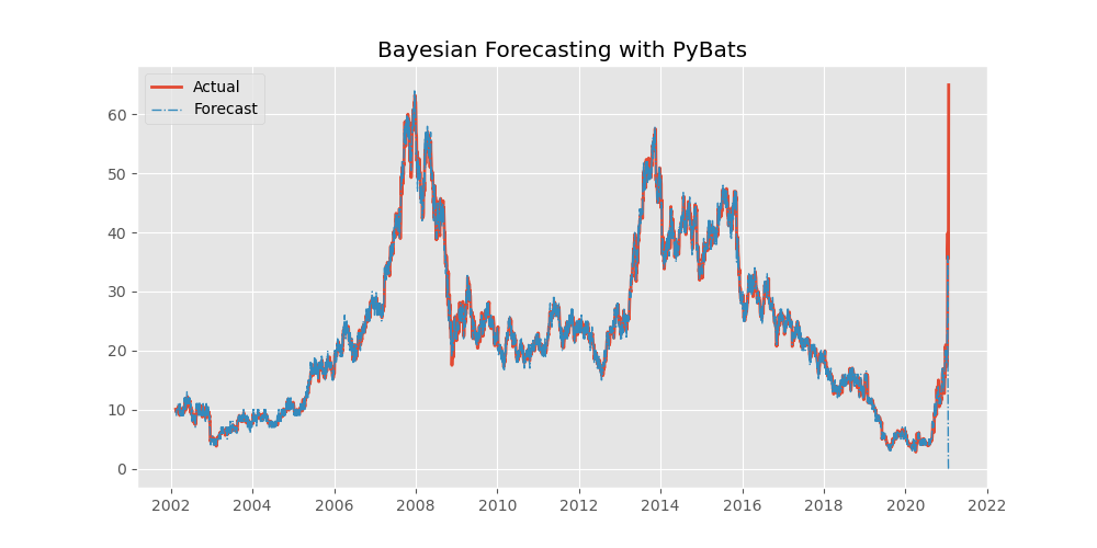
With the forecast executed, we can cast the median of the posterior distribution samples as the point estimate forecast. The code below assigns the index to the respect forecast into a singular dataframe.
forecast = pd.DataFrame(median(samples)[1:], columns=['forecast'])
forecast.index = close_data.index[1:]
fig = plt.figure( figsize=(10, 5))
plt.plot(close_data.index, close_data.close_price, linewidth=2, label='Actual')
plt.plot(forecast.index, forecast.forecast, linestyle='-.', linewidth=1, label='Forecast')
plt.title('Bayesian Forecasting with PyBats')
plt.legend()
plt.show()
def mape(forecast, actual):
        return np.mean( np.abs(forecast - actual)/actual) * 100

mape(forecast.forecast,close_data.close_price)4.160323236448572
Even without specifying time series level components such as trends and seasonality, the forecast on using linear components fits the data incredibly well with the MAPE value of 4.1% on the training dataset.