An Intuitive Introduction to PyTorch with Linear Regression
Deep Learning frameworks such as PyTorch and Tensorflow are specifically crafted to incorporate essential concepts such as model architecture, dataset class, optimizers, and epoch-based training routines, which differ from those found in general machine learning toolkits. Unlike scikit-learn, which heavily abstracts these elements, Pytorch is a class-based tool that may be less intuitive to transition to.
This note introduces the fundamental concepts of Pytorch, utilizing the Simple Linear Regression problem as an example. The note covers the following key concepts:
- 1. Dataset
- 2. DataLoader
- 3. Model Architecture
- 4. Training and Validation Routines
- 5. Model Predictions
A Simple Linear Regression
If you have done any ML modeling, you would be familiar with the Simple Linear Regression technique. With its statistical assumption aside, Simple Linear Regression is a technique used to quantify the linear relation of one variable to an outcome. Think, mileage on a car and its relationship to the price of the car.
Mathematically, SLR is represented as:
$$ y = \alpha + \beta x_i + \epsilon $$
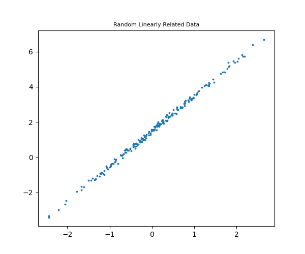
It is helpful to use a simple approach to intuitively discuss Gradient Descent. In this section, we develop data with a linear relationship.
Generating Random Linearly Related Data
In the code below, the true $\alpha$ and $\beta$ parameters are set to $\alpha=1.5$ and $\beta=2.0$. The code generates random $x$ and $\epsilon$ values and uses the formula to generate $y$ values.
import torch
import numpy as np
import matplotlib.pyplot as plt

# Inline Visualization
%matplotlib inline
%config InlineBackend.figure_format = 'retina'
# setting the true parameters
true_alpha, true_beta = 1.5, 2.0
# set seed for reproducibility
torch.manual_seed(420)
# generate random x and epsilon values
x = torch.randn(200, dtype=torch.float)
epsilon = .1 * torch.randn(200, dtype=torch.float)
y = true_alpha + true_beta * x + epsilonplt.figure(figsize=(6, 5))
plt.scatter(x, y, s=3)
plt.title('Random Linearly Related Data', size=8)
plt.show()
1. Dataset Class
Pytorch offers the Dataset class as the primary data storage and access module for both pre-loaded and external datasets. To set a data class, we simply create a class that inherits from Dataset and define two methods.
- 1. __getitem__: To retrieve the data by index
- 2. __len__: To retrieve the size of our data.
Here is an example of a simple LinearData class.
from torch.utils.data import Dataset, DataLoader, random_split

class LinearData(Dataset):

    def __init__(self, x_input, y_output):
        self.x_input = x_input
        self.y_output = y_output


    def __getitem__(self, index):
        if index >= len(self.x_input):
            return "Value Does not exist"
        return (self.x_input[index], self.y_output[index])

    def __len__(self):
        return len(self.x_input)
# initializing data
data = LinearData(x_input=x, y_output=y)
# Getting the size of the data and values of index 5
len(data), data[5](200, (tensor(0.3826), tensor(2.3138)))
2. DataLoader
DataLoader is the utility class that helps us split our data into batches we need for training. Training in batches is common and recommended practice in Deep Learning and the DataLoader class offers the utility to seamlessly integrate Dataset and DataLoaders.
One additional step before using the DataLoader is to split the data into train and test sets. We can do this using the $random\_split()$ method which takes the Dataset class we created above and numerical train and test values.
train_set, test_set = random_split(data, [160, 40])
len(train_set), train_set[5], len(test_set), test_set[5](160, (tensor(-0.2842), tensor(0.9222)), 40, (tensor(2.1325), tensor(5.8129)))
Setting the DataLoader
train_data_loader = DataLoader(dataset=train_set, batch_size=16, shuffle=True)
test_data_loader = DataLoader(dataset=test_set, batch_size=16, shuffle=True)
Model Architecture
Pytorch models are built as architectures inheriting model configurations from the $Module$ class. The $Module$ class has many built-in classes that can be customized for varying complexities across different domains. In this rather simple example, we can implement two linear models: one inherited and another constructed in the model
import torch.nn as nn

# Model with Parameter Initializations
class CustomLinearModel(nn.Module):

    def __init__(self):
        # Initialize nn.Module
        super().__init__()
        self.alpha = nn.Parameter(torch.randn(1, requires_grad=True, dtype=torch.float))
        self.beta = nn.Parameter(torch.randn(1, requires_grad=True, dtype=torch.float))

    def forward(self, x):
        return self.alpha + self.beta * x


# Using the Linear Module
class SimpleLinearModel(nn.Module):

    def __init__(self):
        super().__init__()
        self.linear = nn.Linear(1, 1)

    def forward(self, x):
        return self.linear(x)
Notice that because this is a simple linear regression problem, creating a custom parameter initialization is not a significant hurdle. You can imagine a model with many more parameters, it would be inefficient. The $nn.Linear()$ method is more scalable because it generates the parameters we need based on the input and output dimensions of our datasets.
The code below initializes the models and uses $state_dict$ to access the parameters.
torch.manual_seed(420)

# initialize model
custom_linear_model = CustomLinearModel()
linear_model = SimpleLinearModel()

# show the initialized parameters
custom_linear_model.state_dict(), linear_model.state_dict()(OrderedDict([('alpha', tensor([-1.6977])), ('beta', tensor([0.6374]))]),
OrderedDict([('linear.weight', tensor([[-0.3051]])),
('linear.bias', tensor([-0.6891]))]))4. Training and Validation Routine
Pytorch's training and validation routine centers around 4 key concepts:
- 1. Optimizer configuration
- 2. Loss function initialization
- 3. Gradient Computation and Parameter Updates
- 4. Loss Tracking
4.1 4.1 Optimizer Configuration
Optimizers are responsible for updating parameter values. PyTorch offers several optimizers which use different approaches to update parameters toward loss minimization. Examples of these are SGD (Stochastic Gradient Descent) and Adam. To initialize an optimizer, we pass in the model's initial parameters and learning rate.
import torch.optim as optim

learning_rate = .1
optimizer = optim.SGD( linear_model.parameters(), lr= learning_rate )
4.2 Loss function
Loss functions calculate our measure of fit and quality of parameters. For our SLR model, we will use the MSE (Mean Square Errors) Loss function.
# loss function
mse_loss = nn.MSELoss(reduction='mean')
4.3 Gradient Computation and Parameter Updates
The gradient computing and parameter updating happen sequentially within the training loop. We will see these in action in the complete training loop but the steps are:
- 1. Compute loss
- 2. Compute gradient
- 3. Update parameters.
# computes gradients
mse_loss.backward()

# update parameters
optimizer.step()

# Reset gradients
optimizer.zero_grad()
4.4 Loss Tracking
Finally, we can track loss values by simply using a container variable like a list. It is useful to track losses at the mini_batch level as well to better understand the training improvements over the course of model training.
losses = []4.5 Putting the Training Routine Together
Combining the above concepts, we can complete the training routine as seen below.
torch.manual_seed(420)

# initialize model
linear_model =  CustomLinearModel()

learning_rate = .1
epochs = 100

optimizer = optim.SGD( linear_model.parameters(), learning_rate)
mse_loss = nn.MSELoss( reduction='mean' )

losses = []

for epoch in range(epochs):

    mini_batch_losses = []
    for x_batch, y_batch in train_data_loader:

        # set model to training mode
        linear_model.train()


        # generate predictions
        y_pred = linear_model(x_batch)

        # compute loss and gradient
        loss = mse_loss(y_pred, y_batch)
        loss.backward()

        # Update parameters and reset gradients
        optimizer.step()
        optimizer.zero_grad()

        mini_batch_losses.append(loss.item())

    loss = np.mean(mini_batch_losses)
    losses.append(loss)

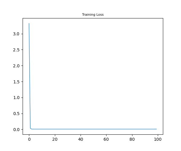
linear_model.state_dict()OrderedDict([('alpha', tensor([1.4954])), ('beta', tensor([2.0015]))])One useful step after model training is to visualize the loss trend with every training epoch. Because the losses variable tracks avg loss per epoch, visualizing loss over time is simplified.
plt.figure(figsize=(6, 5))
plt.plot(losses, linewidth=1)
plt.title("Training Loss", size=8)
plt.show()
5. Model Predictions
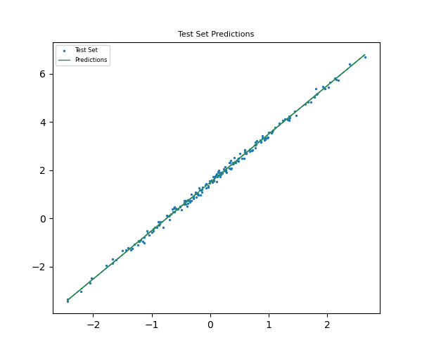
To run model predictions, the model object must be set to evaluate mode before passing in the inputs for prediction.
linear_model.eval()
test_predictions = linear_model(test_set.dataset.x_input)
plt.figure(figsize=(6, 5))
plt.scatter(test_set.dataset.x_input, test_set.dataset.y_output, label="Test Set", s=2)
plt.plot(test_set.dataset.x_input, test_predictions.detach().numpy(), color="seagreen", label="Predictions", linewidth=1)
plt.title("Test Set Predictions", size=8)
plt.legend(fontsize="6")
plt.show()
Additional Concepts
This note covers foundational concepts for using Pytorch. However, there are some steps not included in this note such as validation loss tracking, model checkpoints, and saving. Similarly, most training pipelines that you will see out there utilize class-based designs that abstract individual components of the training routines. These will be discussed as we get into more advanced Deep Learning Architectures.